

Community hub
Recent from talks
Contribute something
Nothing was collected or created yet.
G banding
View on Wikipedia
G-banding, G banding or Giemsa banding is a technique used in cytogenetics to produce a visible karyotype by staining condensed chromosomes. It is the most common chromosome banding method.[1] It is useful for identifying genetic diseases (mainly chromosomal abnormalities) through the photographic representation of the entire chromosome complement.[2]
Method
[edit]The metaphase chromosomes are treated with trypsin (to partially digest the chromosome) and stained with Giemsa stain. Heterochromatic regions, which tend to be rich with adenine and thymine (AT-rich) DNA and relatively gene-poor, stain more darkly in G-banding. In contrast, less condensed chromatin (Euchromatin)—which tends to be rich with guanine and cytosine (GC-rich) and more transcriptionally active—incorporates less Giemsa stain, and these regions appear as light bands in G-banding.[3] The pattern of bands are numbered on each arm of the chromosome from the centromere to the telomere. This numbering system allows any band on the chromosome to be identified and described precisely.[4] The reverse of G‑bands is obtained in R‑banding. Staining with Giemsa confers a purple color to chromosomes, but micrographs are often converted to grayscale to facilitate data presentation and make comparisons of results from different laboratories.[5]
The less condensed the chromosomes are, the more bands appear when G-banding. This means that the different chromosomes are more distinct in prophase than they are in metaphase.[6]
-
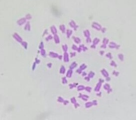 Micrograph of human male chromosomes using Giemsa staining for G banding.
 -
 Micrograph of human male chromosomes using Giemsa stain, followed by sorting and grayscaling.
.jpg)

Advantage
[edit]It is difficult to identify and group chromosomes based on simple staining because the uniform colour of the structures makes it difficult to differentiate between the different chromosomes. Therefore, techniques like G‑banding were developed that made "bands" appear on the chromosomes. These bands were the same in appearance on the homologous chromosomes, thus, identification became easier and more accurate.
Types of banding
[edit]Other types of cytogenic banding are listed below:
| Banding type | Staining method |
|---|---|
| C-banding | Constitutive heterochromatin |
| G-banding | Giemsa stain |
| Q-banding | Quinacrine |
| R-banding | Reverse Giemsa staining |
| T-banding | Telomeric |
See also
[edit]References
[edit]- ^ Maloy, Stanley R.; Hughes, Kelly (2013). Brenner's encyclopedia of genetics. San Diego, CA. ISBN 978-0-08-096156-9. OCLC 836404630.
{{cite book}}: CS1 maint: location missing publisher (link) - ^ Speicher, Michael R. and Nigel P. Carter. "The New Cytogenetics: Blurring the Boundaries with Molecular Biology." Nature Reviews Genetics, Vol 6. Oct 2005.
- ^ Romiguier J, Roux C (2017). "Analytical Biases Associated with GC-Content in Molecular Evolution". Front Genet. 8: 16. doi:10.3389/fgene.2017.00016. PMC 5309256. PMID 28261263.
- ^ Nussbaum, Robert; McInnes, Roderick; Willard, Huntington (2015). Thompson & Thompson, Genetics in Medicine (Eighth ed.). Canada: Elsevier Inc. p. 58. ISBN 978-1-4377-0696-3.
- ^ Lee M. Silver (1995). Mouse Genetics, Concepts and Applications. Chapter 5.2: KARYOTYPES, CHROMOSOMES, AND TRANSLOCATIONS. Oxford University Press. Revised August 2004, January 2008
- ^ Nussbaum, McInnes, Willard (21 May 2015). Genetics in Medicine. Elsevier. pp. 57–73. ISBN 978-1-4377-0696-3.
{{cite book}}: CS1 maint: multiple names: authors list (link)
G banding
View on GrokipediaIntroduction
Definition and Principle
G banding, also known as Giemsa banding, is a cytogenetic staining technique used to produce a visible karyotype by revealing characteristic alternating dark and light bands along the length of metaphase chromosomes. This method, first described in 1971, enables the identification and analysis of individual chromosomes by highlighting their structural features under a light microscope. The underlying principle of G banding involves pretreatment of fixed chromosomes with a proteolytic enzyme such as trypsin or mild heat to partially denature and remove some chromosomal proteins, exposing underlying DNA structures. Subsequent staining with Giemsa dye, a complex mixture, results in differential binding that produces dark G-positive bands in regions of constitutive heterochromatin and light G-negative bands in euchromatic areas. Dark bands correspond to gene-poor, late-replicating DNA sequences that are AT-rich, while light bands represent gene-rich, early-replicating regions that are GC-rich. At the biochemical level, Giemsa stain comprises azure B (a thiazine dye derived from methylene blue), eosin, and methylene blue, which interact specifically with chromosomal components.[6] The azure B component binds preferentially to the phosphate groups of AT-rich DNA in heterochromatic regions, while eosin associates with basic proteins, enhancing contrast after pretreatment disrupts protein-DNA interactions and exposes band-specific chromatin conformations.[7] This selective affinity, influenced by base composition and chromatin compaction, underlies the banding pattern's visibility. G banding typically achieves a resolution of 5-10 megabases, allowing detection of chromosomal abnormalities at the level of large-scale rearrangements but not smaller submicroscopic changes.[8]Role in Cytogenetics
G banding serves as the standard method in cytogenetics for visualizing the full set of 46 human chromosomes in metaphase spreads, enabling the detection of both numerical and structural abnormalities through its characteristic banding patterns.[9] This technique allows cytogeneticists to arrange chromosomes into a karyogram, facilitating precise identification and analysis of the human genome at the chromosomal level.[10] By producing reproducible, species-specific patterns, G banding has become integral to routine karyotyping workflows in clinical and research settings.[11] In genetic diagnosis, G banding plays a pivotal role in identifying key chromosomal aberrations, such as aneuploidies and translocations. For instance, it reveals trisomy 21, characterized by an extra chromosome 21, which is diagnostic for Down syndrome.[12] Similarly, G banding detects the Philadelphia chromosome, resulting from the t(9;22)(q34;q11.2) translocation, in approximately 90% of chronic myeloid leukemia (CML) cases, aiding in disease confirmation and prognosis assessment.[13] These capabilities have made G banding essential for diagnosing constitutional and acquired genetic disorders. G banding evolved from earlier uniform or solid staining techniques, such as basic Giemsa staining without pretreatment, which provided only gross morphological details without distinct patterns for chromosome differentiation.[4] The introduction of trypsin pretreatment followed by Giemsa staining in the early 1970s markedly improved resolution, allowing pattern-specific identification of individual chromosomes and subtle structural changes that were previously undetectable.[1] Despite advancements in molecular cytogenetic methods like fluorescence in situ hybridization (FISH) and array comparative genomic hybridization (array CGH), which offer higher resolution for submicroscopic alterations, G banding remains the gold standard for genome-wide chromosome analysis due to its cost-effectiveness, accessibility, and ability to detect balanced rearrangements and low-level mosaicism.[14] It continues to be recommended as the initial screening tool in prenatal and postnatal diagnostics, often complemented by molecular techniques for comprehensive evaluation.[15]Historical Development
Early Discoveries in Chromosome Banding
The discovery of chromosomes traces back to 1842, when Swiss botanist Karl Wilhelm von Nägeli first observed thread-like structures in pollen mother cells of plants using light microscopy.[16] This initial identification laid the groundwork for cytological studies, though the structures were not yet recognized as bearers of hereditary information. In the ensuing decades, early visualization efforts relied on basic dyes to enhance contrast; hematoxylin, derived from the heartwood of Haematoxylum campechianum, emerged as a key nuclear stain in the mid-19th century, allowing microscopists to differentiate cellular components more clearly despite its non-specific binding.[17] These rudimentary staining techniques, often combined with mordants like alum, enabled the observation of chromosomes in animal and plant cells but produced uniform coloration that obscured fine structural details.[18] Advancements in the 1950s and 1960s transformed chromosome preparation by addressing preparation challenges to achieve clearer spreads. The introduction of colchicine, a mitotic inhibitor derived from the autumn crocus, arrested cells in metaphase, where chromosomes are maximally condensed and visible, significantly increasing the yield of analyzable metaphase figures.[19] Concurrently, hypotonic treatment—exposing cells to a dilute salt solution—swelled them, facilitating separation of chromosomes from the mitotic spindle and cytoplasm for better spreading on slides.[20] These methods culminated in the seminal 1956 study by Joe Hin Tjio and Albert Levan, who applied them to human cells and definitively established the diploid chromosome number as 46, correcting prior erroneous counts of 48.[20] Their work, using cultured fibroblasts and direct bone marrow preparations, demonstrated how these techniques enabled reliable enumeration and morphological assessment across species.[19] The concept of chromosome banding emerged in the late 1960s as a breakthrough to overcome the limitations of uniform staining, which had long hindered individual chromosome identification. In 1969, Lore Zech reported the first differential banding patterns using quinacrine mustard, a fluorescent acridine derivative that binds preferentially to adenine-thymine-rich DNA regions, producing bright, heterogeneous fluorescence under UV light—known as Q-banding.[1] This technique revealed distinct patterns on human chromosomes, particularly highlighting the Y chromosome's intense fluorescence, allowing for the first time the unequivocal distinction of all chromosome pairs without relying solely on size or shape. Prior to such methods, uniform staining with dyes like aceto-orcein or Feulgen had rendered many chromosomes morphologically indistinguishable, complicating karyotyping and aberration detection in clinical and research settings.[21]Invention of G Banding
The G-banding technique was independently developed in 1971 by multiple research groups, marking a pivotal advancement in chromosome visualization. Among the earliest reports, Maximo E. Drets and Margery W. Shaw described a method involving alkali treatment with NaOH, followed by incubation in a sodium chloride-trisodium citrate buffer and Giemsa staining, which produced distinct banding patterns on human metaphase chromosomes. Concurrently, S.R. Patil, S. Merrick, and H.A. Lubs introduced a simplified protocol using a modified Giemsa stain after brief exposure to a phosphate buffer, enabling clear identification of individual human chromosomes. The discovery of G-banding often stemmed from serendipitous observations during experiments aimed at other staining methods. For instance, Marina Seabright's seminal work on the trypsin pretreatment method originated from an accidental contamination with trypsin in a 1967 chromosome preparation, which revealed banding-like stripes dismissed as artifacts at the time; by 1971, she refined this into a reproducible technique involving brief trypsin digestion to partially remove chromosomal proteins, followed by Giemsa staining, allowing rapid and consistent band resolution under a light microscope.[22] Similarly, A.T. Sumner, H.J. Evans, and R.A. Buckland developed a straightforward procedure using incubation in a 2x SSC saline solution prior to Giemsa staining, which also yielded high-contrast G-bands and was particularly effective for distinguishing human chromosomes. These innovations evolved from earlier Q-banding techniques, which relied on fluorescent quinacrine stains but required specialized equipment; G-banding offered the advantage of permanent, non-fluorescent stains compatible with standard light microscopy, broadening accessibility. The technique's initial methods, such as protein digestion via trypsin or alkaline denaturation, were first reproducible in these 1971 protocols, transforming cytogenetic analysis by revealing longitudinal chromosome differentiation.[23] Standardization occurred at the Paris Conference on Standardization in Human Cytogenetics in 1971, where participants, including representatives from the discovering groups, adopted G-banding as a core method and established foundational nomenclature for band patterns, laying the groundwork for the International System for Human Cytogenomic Nomenclature (ISCN). This conference recognized the collective contributions of key figures like Drets, Shaw, Seabright, Patil, and Sumner, ensuring G-banding's integration into routine karyotyping.Procedure
Safety precautions must be observed throughout the procedure, including wearing appropriate personal protective equipment (PPE) such as gloves, lab coat, and eye protection; performing fixative and staining steps in a fume hood; handling biological samples as biohazards; and disposing of chemical and biological waste according to institutional and regulatory guidelines.[24]Chromosome Preparation
Chromosome preparation for G-banding begins with the selection and processing of appropriate cell sources to obtain high-quality metaphase spreads. Common samples include peripheral blood lymphocytes, which are easily accessible and stimulated for division; amniotic fluid cells from prenatal diagnostics; and tumor biopsies for cancer cytogenetics. For peripheral blood, 0.5–1 mL of heparinized whole blood is inoculated into 10 mL of RPMI-1640 medium supplemented with 15–20% fetal bovine serum, antibiotics, and 1–2% phytohemagglutinin (PHA) as a mitogen to induce lymphocyte proliferation. The culture is incubated at 37°C in 5% CO₂ for 72 hours to accumulate dividing cells. Amniotic fluid cells are similarly cultured in Chang medium or equivalent for 7–10 days until confluent, while tumor samples may require short-term culture or direct harvest depending on the tissue type and viability.[24][25] To arrest cells in metaphase, a spindle poison such as colchicine or Colcemid (demecolcine) is added to depolymerize microtubules and halt progression at this stage, where chromosomes are maximally condensed and visible. For peripheral blood lymphocytes, Colcemid is typically used at a final concentration of 0.02–0.1 µg/mL for 0.5–2 hours at 37°C, though ranges of 0.02–0.05 µg/mL for 1–3 hours are also standard to balance arrest efficiency and chromosome length. Similar conditions apply to cultured amniotic or tumor cells, adjusted for proliferation rate—shorter times for rapidly dividing lines to avoid over-contraction. After treatment, cells are centrifuged at 200–300 × g for 5–10 minutes to collect the pellet.[24][27] Hypotonic swelling follows to increase cell volume, disrupt the cytoplasm, and facilitate chromosome dispersion. The cell pellet is gently resuspended in prewarmed 0.075 M KCl solution at 37°C, typically 5–10 mL per culture flask, and incubated for 10–30 minutes to achieve optimal swelling without chromosome loss. This step is critical for producing well-spread metaphase plates; shorter times (10–15 minutes) suit blood lymphocytes, while longer incubations (20–30 minutes) may benefit denser tumor preparations. Excess hypotonic solution is removed by centrifugation before proceeding.[24][27] Fixation preserves chromosome morphology by dehydrating and stabilizing the spreads. Ice-cold fixative, usually a 3:1 mixture of methanol to glacial acetic acid (Carnoy's solution), is added dropwise to the swollen cells while vortexing gently to avoid clumping—initially 5 mL, followed by additional volumes to reach 10–15 mL total. The suspension is left at 4°C for 10–30 minutes, then centrifuged, and the process repeated 2–3 times with fresh fixative (6–8 mL each) until the supernatant is clear, ensuring removal of cytoplasmic residues. For amniotic or tumor cells, up to 4–5 changes may be needed if lipids are present. The final fixed cell suspension is stored at -20°C or used immediately.[24][27] Slide preparation involves depositing the fixed cells onto glass slides to create monolayer spreads suitable for banding. A small volume (3–5 drops) of the suspension is dropped from a height of 2–3 inches onto a clean, wet slide tilted at 45° under humid conditions to control spreading; humidity (50–60%) and temperature (20–25°C) influence droplet evaporation and chromosome dispersion. Slides are air-dried gradually, then aged at room temperature for days to weeks to enhance adhesion and banding quality, or briefly baked at 60°C for 2–18 hours if immediate use is required. Optimal aging promotes even distribution of metaphases without overlap, crucial for subsequent visualization.[24][25][27]Staining and Visualization
The staining and visualization process in G banding begins with a pretreatment step to partially digest chromosomal proteins, enhancing the differential uptake of the stain. The most common pretreatment involves brief exposure to trypsin, typically at a concentration of 0.025-0.05% in a saline solution (such as 0.9% NaCl or phosphate-buffered saline at pH 7.2-7.4), for 10 seconds to 2 minutes at room temperature or 37°C, depending on slide age and enzyme activity.[28][29][30] Following pretreatment, slides are rinsed in saline or buffer to halt the reaction and prevent over-digestion. The core staining step employs Giemsa solution, a mixture of methylene blue, eosin, and azure B dyes, applied at 2-6% concentration in a phosphate buffer (typically Sorensen's or Gurr's at pH 6.8) for 5-10 minutes at room temperature.[28][30][31] This duration and concentration may be adjusted based on stain batch variability, with some protocols adding a small volume of acetone (e.g., 1-2%) to modulate staining intensity. After staining, slides are rinsed briefly in the same pH 6.8 buffer or distilled water to remove excess dye, air-dried, and mounted with a coverslip using a medium like Permount or Cytoseal 60, often followed by brief heating at 50-60°C to set the preparation.[28][32][30] Visualization occurs under a bright-field light microscope, where metaphase spreads are examined at magnifications ranging from 400x to 1000x, often using a 40x or 100x oil-immersion objective for optimal resolution of band patterns.[33][30] The Giemsa stain produces alternating dark (G-positive, AT-rich regions) and light (G-negative, GC-rich regions) bands along each chromosome, yielding a resolution of 400-850 bands per haploid genome set, with higher numbers (up to 850) achievable under optimal conditions for detailed analysis.[34] Quality control is essential to ensure band sharpness and contrast, assessed visually during initial microscopic inspection. Over-trypsinization or excessive heat can result in fuzzy, poorly defined bands due to over-digestion of chromosomal proteins, while under-treatment leads to uniform staining with insufficient contrast between bands; adjustments to pretreatment time or enzyme concentration are made iteratively on test slides to optimize results.[27][33][35]Interpretation of Results
Banding Patterns
G banding produces a distinctive alternating pattern of dark and light bands along the length of metaphase chromosomes, enabling the identification of individual chromosomes within the human karyotype. Dark G bands, also known as G-positive bands, appear as densely stained regions that are AT-rich, relatively gene-poor, and associated with more condensed heterochromatin-like structures. In contrast, light G bands, or G-negative bands, stain more faintly and correspond to GC-rich, gene-dense euchromatic regions that are less condensed.[36][37][2] These banding patterns have clear biological correlates tied to DNA replication timing and chromatin function. Dark G bands replicate late during the S-phase of the cell cycle and are enriched in repetitive DNA sequences, contributing to their condensed state and reduced transcriptional activity. Light G bands, conversely, replicate early in S-phase and harbor actively transcribed genes, including housekeeping genes essential for basic cellular functions, while tissue-specific genes are more commonly found in dark bands. This replication timing dichotomy aligns with the compositional differences, where the GC-rich nature of light bands supports higher gene density and accessibility for transcription.[38][39][2] The resolution and visibility of G banding patterns vary depending on the degree of chromosome condensation during metaphase arrest; less condensed chromosomes yield higher resolution with more discernible sub-bands, while overly condensed ones reduce detail. Standard G banding protocols typically resolve approximately 550 bands across the haploid complement (one set of 23 chromosomes), providing sufficient detail for routine cytogenetic analysis, though advanced techniques can achieve up to 850 bands or more under optimized conditions.[40][36] True G banding patterns must be distinguished from artifacts arising from non-specific staining, which can occur due to suboptimal trypsin digestion or Giemsa application, leading to uneven or hazy bands that mimic pathological changes. For instance, excessive staining at telomeres or centromeres may result from residual heterochromatin binding rather than genuine G-positive regions, necessitating multiple metaphase spreads for confirmation to rule out technical variability.[36][33]Nomenclature and Karyotyping
The International System for Human Cytogenomic Nomenclature (ISCN) provides a standardized framework for designating G-banded chromosomes and their structural features.[41] Each band is identified by a hierarchical notation starting with the chromosome number, followed by the arm designation (p for the short arm or q for the long arm), the region number, the band number, and optional sub-band levels for higher resolution (e.g., 21q22.13, which specifies the critical region on the long arm of chromosome 21 associated with Down syndrome phenotypes).[42] This system, originally developed for G-banding patterns, allows precise localization of chromosomal abnormalities such as deletions, duplications, or translocations by referencing idiograms—diagrammatic representations of G-banded karyotypes that illustrate band levels and heterochromatic regions.[43] In karyotype assembly, G-banded chromosomes from a metaphase spread are photographed, cut out, and systematically arranged into 23 pairs based on size, centromere position, and banding patterns, resulting in a display of the full 46-chromosome complement for humans.[44] At least 20 well-banded metaphases are typically analyzed to ensure reliability and detect potential mosaicism, where a subset of cells exhibits a different karyotype.[44] This process facilitates the identification of numerical aberrations (e.g., aneuploidy) or structural variants by comparing observed patterns against ISCN ideograms. Digital imaging systems have streamlined karyotyping by automating chromosome capture, segmentation, classification, and arrangement from G-banded slides, significantly reducing manual effort while maintaining accuracy through operator oversight.[45] Tools such as Ikaros software integrate real-time microscope imaging to generate karyograms, and emerging AI algorithms further enhance auto-karyotyping by processing metaphase images for abnormality prediction, though manual verification remains essential to resolve ambiguities in band interpretation.[46] The ISCN has evolved iteratively since its inception at the 1971 Paris Conference, which established the foundational nomenclature for cytogenetic reporting, through 11 editions that adapt to advancing technologies.[41] Early versions focused on banding techniques like G-banding, but the 2020 edition incorporated cytogenomic elements, with the 2024 update introducing standardized rules for integrating molecular data such as microarray and sequencing results alongside traditional band notations to support comprehensive genomic descriptions.[41]Advantages and Limitations
Advantages
G-banding offers high resolution and specificity in cytogenetic analysis, enabling the reliable distinction of all 22 autosomes and the sex chromosomes through characteristic banding patterns that correspond to regions of varying guanine-cytosine content.[47] This technique can detect structural abnormalities such as deletions and duplications larger than 5–10 megabases (Mb), which is sufficient for identifying many clinically significant chromosomal variants without requiring prior knowledge of specific genetic targets.[48] The method is highly cost-effective, relying on basic laboratory equipment including a light microscope and standard Giemsa staining reagents, without the need for specialized fluorescence microscopy or advanced molecular tools.[2] Its simplicity and low material costs make it accessible for routine use in diverse clinical and research settings worldwide. G-banding provides a comprehensive, genome-wide view of chromosomal integrity in a single assay, allowing simultaneous evaluation of numerical abnormalities (e.g., aneuploidy) and structural variants such as translocations and inversions across the entire karyotype.[47] Stained preparations from G-banding are permanent and stable for years when properly stored, facilitating long-term archival and repeated examinations without signal degradation, in contrast to fluorescent-based methods.[47]Limitations
G-banding, while a foundational technique in cytogenetics, has inherent resolution constraints that limit its ability to detect submicroscopic chromosomal alterations. Specifically, it cannot identify deletions, duplications, or rearrangements smaller than approximately 5-10 megabases (Mb), nor can it detect point mutations or single nucleotide variants.[49][50] This resolution threshold means that balanced translocations or inversions lacking a clear phenotypic impact—particularly those below the detectable size—may go unnoticed, as the banding patterns remain visually unaltered.[2] Another significant drawback is the technique's dependence on cells in metaphase, requiring active proliferation and culturing to obtain sufficient dividing cells for analysis. This poses challenges for tissues with low mitotic activity, such as non-proliferative samples or solid tumors, where obtaining adequate metaphases is often difficult or impossible without extended culture periods.[51] In such cases, the scarcity of suitable metaphases can lead to incomplete or failed analyses.[52] The process is labor-intensive and prone to subjectivity, involving manual chromosome preparation, staining, and microscopic interpretation that can take several days for cell culture and processing alone.[33] Band-level estimation and abnormality identification vary between observers, introducing interpretive inconsistencies that affect diagnostic reliability.[53][54] Furthermore, in vitro culturing introduces potential artifacts, including biased cell selection that may not represent the original tissue composition and underrepresentation of mosaicism due to uneven proliferation rates among cell populations.[55][56] This can result in misleading karyotypes, particularly in heterogeneous samples like tumors or gonadal tissues, where cultured cells might not accurately reflect in vivo genetics.[57]Applications
Clinical Diagnostics
G-banding, a standard cytogenetic technique involving Giemsa staining to produce characteristic light and dark bands on chromosomes, is integral to prenatal screening for fetal chromosomal abnormalities. It is routinely applied to samples obtained via amniocentesis, typically performed between 15 and 20 weeks of gestation, or chorionic villus sampling (CVS) at 10-13 weeks, to provide definitive diagnosis following positive screening results from noninvasive prenatal testing (NIPT). This method enables visualization of whole chromosome aneuploidies, such as trisomy 18 (Edwards syndrome) and trisomy 13 (Patau syndrome), which are associated with severe developmental issues and high rates of fetal loss. Additionally, G-banding can detect larger structural rearrangements, though its resolution is limited to abnormalities larger than 5-10 Mb.[58] In postnatal diagnostics, G-banding serves as a primary tool for confirming constitutional chromosomal abnormalities in individuals presenting with dysmorphic features, growth delays, or intellectual disabilities. For Turner syndrome, characterized by a 45,X karyotype in approximately 50% of cases, G-banding analysis of peripheral blood lymphocytes identifies the monosomy X, distinguishing it from mosaic variants and guiding management for associated cardiac and renal anomalies. Similarly, in Cri-du-chat syndrome, G-banding detects the partial deletion of the short arm of chromosome 5 (5p15.2-p15.3), confirming the diagnosis in infants with the distinctive high-pitched cry, microcephaly, and hypotonia; the technique delineates deletion size to correlate with phenotypic severity. These analyses typically involve analyzing at least 20 metaphases to ensure accuracy.[59][60] Cancer cytogenetics relies heavily on G-banding to identify acquired clonal abnormalities that inform prognosis and therapy in hematologic malignancies. In chronic myeloid leukemia (CML), G-banding detects the hallmark t(9;22)(q34;q11.2) Philadelphia chromosome in over 95% of cases, enabling risk stratification when additional abnormalities like trisomy 8 or i(17q) are present, which indicate progression to blast crisis. For acute myeloid leukemia (AML) and lymphomas, such as chronic lymphocytic leukemia or non-Hodgkin lymphoma, G-banding at diagnosis analyzes bone marrow or lymph node metaphases to uncover recurrent translocations (e.g., t(8;14) in Burkitt lymphoma) or numerical changes, supporting targeted treatments like tyrosine kinase inhibitors in CML. The American College of Medical Genetics and Genomics (ACMG) standards mandate G-banded analysis of at least 20 cells for initial diagnostics, with results integrated into the World Health Organization classification of tumors.[61][62] Professional guidelines from the American College of Obstetricians and Gynecologists (ACOG) and ACMG endorse G-banding as the foundational method for initial karyotyping in suspected chromosomal disorders across prenatal, postnatal, and oncology settings. ACOG recommends offering invasive diagnostic testing with G-banded karyotyping to all patients with abnormal screening results, emphasizing informed consent and genetic counseling to weigh miscarriage risks (0.5-1%) against diagnostic certainty. ACMG advises routine G-banding at 400-550 band resolution for evaluating intellectual disability or congenital anomalies, positioning it as the first-line cytogenetic test before advanced methods like chromosomal microarray if needed. These recommendations ensure standardized workflows for timely clinical decision-making.[58][63]Research and Other Uses
G-banding has been instrumental in evolutionary studies, particularly for comparing chromosome structures across species to identify conserved synteny, which refers to the preservation of gene order on chromosomes despite evolutionary divergence. In mammalian evolution, analyses of G-banded chromosomes have revealed homologous regions between primates and other orders, such as carnivores, highlighting shared ancestral karyotypes and chromosomal rearrangements over time. For instance, detailed G-banding comparisons between human and primate chromosomes, including those of genera like Cebus, have mapped syntenic blocks and inferred phylogenetic relationships, aiding in reconstructing the evolutionary history of chromosomal fusions and inversions.[64][65] In population genetics, G-banding facilitates the assessment of chromosomal polymorphisms, such as heterochromatin variants and inversions, within cohorts to explore ancestry and potential disease risks. Studies of major polymorphisms on chromosomes 1, 9, 16, and Y across ethnic groups, like those in Indian populations, have used G-banding to document frequency differences that correlate with geographic origins and genetic diversity. Additionally, G-banding has identified polymorphic inversions in European ancestry populations, such as the 17q21.31 inversion, which may modulate disease susceptibility by altering gene regulation, providing insights into population-specific genetic risks.[66][67][68] The technique has been adapted for cytogenetic analysis in plants and animals, supporting breeding programs in agriculture and veterinary science. In animal cytogenetics, G-banding screens for chromosomal anomalies in livestock, such as translocations in swine breeding nuclei, enabling the selection of chromosomally stable individuals to improve fertility and productivity. For example, routine G-banding in deer farms has detected Robertsonian translocations associated with infertility, informing targeted breeding strategies to mitigate economic losses. In plant cytogenetics, optimized G-banding protocols, like the SteamDrop method, enhance chromosome preparation for species such as those in Cucurbitaceae, aiding in the identification of karyotypic variations for crop improvement and hybrid development.[69][70][71][72][73] G-banding integrates with modern genomics as a cytogenetic scaffold for aligning sequencing data in hybrid cytogenomic approaches, bridging microscopic and molecular resolutions. By providing a visual reference for large-scale chromosomal architecture, G-banded karyotypes guide the assembly and annotation of genome sequences, particularly in vertebrates where it helps resolve ambiguities in scaffold ordering. This integration has been pivotal in cytogenomics, where G-banding complements techniques like FISH and next-generation sequencing to map structural variants and evolutionary changes at both cytological and genomic levels.[74][75][76]Comparison to Other Banding Techniques
Overview of Other Methods
Q-banding, the first chromosome banding technique developed in 1970 by Torbjörn Caspersson and colleagues, utilizes quinacrine mustard or related fluorochromes to produce fluorescent patterns under UV light.[5] This method highlights AT-rich regions of the genome, where the dye binds preferentially, resulting in bright fluorescence in those areas and dimmer staining elsewhere.[4] Q-banding is particularly valuable for identifying the human Y chromosome due to its prominent brightly fluorescent distal segment on the long arm.[5] R-banding, developed shortly after Q-banding, involves heat denaturation of chromosomes in a saline solution followed by Giemsa staining, producing a reverse pattern compared to G-banding.[77] This technique emphasizes GC-rich euchromatic regions, which appear as dark bands, making it complementary to G-banding for analyzing gene-dense areas, especially near telomeres.[5] C-banding specifically targets constitutive heterochromatin, such as centromeric regions and satellite stalks, by treating chromosomes with alkali or acid to denature DNA and then staining with Giemsa.[78] It reveals blocks of repetitive DNA sequences but offers low resolution for distinguishing euchromatic bands, limiting its utility for detailed karyotyping beyond heterochromatin characterization.[78] Other variants include T-banding, which modifies R-banding procedures to intensely stain telomeric regions while faintly revealing the rest of the chromosome, aiding in end-specific analysis.[79] Extensions of G-banding, such as high-resolution techniques using synchronization agents like methotrexate, allow visualization of sub-bands (up to 850 or more per haploid set) for finer structural detection without altering the core Giemsa-based mechanism.[80]Key Differences
G-banding differs from Q-banding primarily in its staining mechanism and permanence. While Q-banding relies on quinacrine-based fluorescent dyes that require UV microscopy and produce patterns that fade over time, G-banding uses Giemsa stain following trypsin treatment to create stable, non-fluorescent bands observable under standard bright-field microscopy.[36] This makes G-banding preferable for routine karyotyping due to its durability and ease of use, whereas Q-banding is better suited for detecting specific polymorphisms, such as those on the Y chromosome.[4] In comparison to R-banding, G-banding exhibits a reverse pattern where dark G-bands (AT-rich, late-replicating regions) correspond to light R-bands, and vice versa for the GC-rich, early-replicating areas.[81] R-banding, achieved through heat denaturation and Giemsa staining, provides enhanced detail in the gene-rich telomeric and p-arm regions, making it valuable for targeted analyses in European laboratories, while G-banding serves as the global standard for comprehensive chromosome identification and abnormality detection.[36] Unlike C-banding, which selectively stains constitutive heterochromatin—particularly centromeric and pericentromeric regions rich in repetitive DNA—G-banding visualizes a broader array of euchromatic bands across the chromosome arms.[4] This euchromatin focus allows G-banding to detect a wider range of structural abnormalities, such as translocations and deletions, rendering it more versatile for general diagnostics, whereas C-banding is limited to heterochromatin variations with minimal clinical utility today.[81] In modern cytogenetics, G-banding is often complemented by fluorescence in situ hybridization (FISH), which offers higher resolution for submicroscopic changes down to individual genes, compared to G-banding's limit of 5–10 megabases.[36] Despite this, G-banding remains the first-line technique for its cost-effectiveness, ability to survey the entire genome in a single preparation, and established role in initial screening before escalating to FISH or spectral karyotyping for confirmation.[4]References
- https://www.thermofisher.com/us/en/home/references/protocols/[immunology](/page/Immunology)/immunology-protocols/preparation-of-peripheral-blood-cells-for-chromosome-analysis.html