



Community hub
Westgard rules
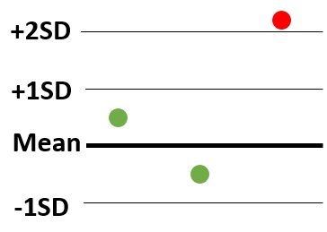
View on WikipediaThe Westgard rules are a set of statistical patterns, each being unlikely to occur by random variability, thereby raising a suspicion of faulty accuracy or precision of the measurement system. They are used for laboratory quality control, in "runs" consisting of measurements of multiple samples. They are a set of modified Western Electric rules, developed by James Westgard and provided in his books and seminars on quality control.[1] They are plotted on Levey–Jennings charts, wherein the X-axis shows each individual sample, and the Y-axis shows how much each one differs from the mean in terms of standard deviation (SD). The rules are:[2]
| Rule | Criteria | Suspected | Example |
|---|---|---|---|
| 12s | One measurement exceeds 2 standard deviations either above or below the mean of the reference range. | Inaccuracy and/or imprecision | 
|
| 13s | One measurement exceeds 3 standard deviations either above or below the mean of the reference range. | Inaccuracy and/or imprecision | 
|
| 22s | 2 consecutive measurements exceed 2 standard deviations of the reference range, and on the same side of the mean. | Inaccuracy and/or imprecision | 
|
| R4s | Two measurements in the same run have a 4 standard deviation difference (such as one exceeding 2 standard deviations above the mean, and another exceeding 2 standard deviations below the mean). | Imprecision. | 
|
| 41s | 4 consecutive measurements exceed 1 standard deviation on the same side of the mean. | Inaccuracy. | 
|
| 10x | 10 consecutive measurements are on the same side of the mean. | Inaccuracy. | 
|
The recommended consequences when any of the above patterns occur is to reject the run, except for the rule of 12s (top in table), which serves as a warning and a recommendation of careful inspection of the data.[2]
See also
[edit]References
[edit]- ^ Ofer Harel; Enrique F. Schisterman; Albert Vexler & Marcus D. Ruopp (July 2008). "Monitoring Quality Control: Can We Get Better Data?". Epidemiology. 19 (4): 621. doi:10.1097/ede.0b013e318176bfb2. PMC 2625303. PMID 18496467.
- ^ a b Heidi Hanes. "Westgard Rules - Guidelines". SMILE, Johns Hopkins University. Review date: 1 April 2020
External links
[edit]Westgard rules
View on Grokipedia- 1_{3s}: Reject the run if one control measurement exceeds the mean ±3s; detects large random or systematic errors.[1]
- 2_{2s}: Reject if two consecutive control measurements exceed the same side of the mean ±2s; indicates systematic error.[1]
- R_{4s}: Reject if one control exceeds +2s and another exceeds -2s within the same run; flags random errors.[1]
- 4_{1s}: Reject if four consecutive measurements exceed the same side of the mean ±1s; identifies trends.[1]
- 10 \bar{x}: Reject if ten consecutive measurements fall on one side of the mean; signals a shift in the process.[1]
- 1_{2s}: A warning rule (not for rejection alone) if one control exceeds ±2s, prompting review of other rules.[1]
Background
Definition and Purpose
Westgard rules constitute a multirule quality control (QC) procedure designed for clinical laboratories, employing a set of statistical decision criteria to assess the acceptability of analytical runs by identifying patterns indicative of out-of-control conditions in measurement processes.[4] This approach integrates multiple rules to evaluate control data, distinguishing it from single-rule systems by providing a more nuanced analysis of variability in laboratory assays.[3] The primary purpose of Westgard rules is to enhance the detection of systematic and random analytical errors while simultaneously reducing false rejections, which could otherwise disrupt laboratory workflows without improving patient safety.[5] By applying these rules to runs involving multiple control samples—typically two to four measurements per run—they enable laboratories to maintain high reliability in test results, supporting accurate clinical decision-making for diagnosis, screening, and monitoring.[4] This balance is critical in high-volume settings where unnecessary halts in reporting could delay patient care. In clinical chemistry and related disciplines, Westgard rules are routinely used to monitor internal QC data against established limits of mean ± standard deviation (SD), ensuring that analytical performance remains stable and deviations are promptly addressed.[6] These rules are often implemented alongside visual tools like Levey-Jennings charts for plotting control values, facilitating the interpretation of trends in precision and accuracy.[3]Historical Development
The Westgard rules were developed by James O. Westgard, a clinical chemist and professor at the University of Wisconsin, in response to quality control challenges faced by clinical laboratories during the 1970s. These challenges arose from the rapid adoption of automated multichannel analyzers, which increased the number of tests per run and led to high false rejection rates—up to 18% in some systems with four controls—when using traditional single-rule procedures like the 2 SD limits.[7][8] Westgard's work was influenced by industrial quality control practices, which he studied during a sabbatical at Uppsala University in 1976–1977, aiming to optimize error detection while minimizing unnecessary rejections.[8] The rules were first formally described in 1981 in the journal Clinical Chemistry (volume 27, issue 3, pages 493–501), in the seminal paper "A multi-rule Shewhart chart for quality control in clinical chemistry" co-authored by Westgard, Patricia L. Barry, Marian R. Hunt, and Torgny Groth. This publication introduced an efficient multirule procedure based on Shewhart control charts, initially designed for two control levels per analytical run to facilitate the transition from simplistic single-rule systems to more robust multi-rule approaches in laboratories.[7][8] Over the following decades, the rules evolved to accommodate varying run sizes, with adaptations for three (N=3) or four (N=4) control measurements per run, enhancing sensitivity to systematic and random errors without excessive false alarms.[7] By the 1990s, the Westgard rules had gained widespread adoption, becoming integrated into guidelines from organizations such as the Clinical and Laboratory Standards Institute (CLSI), where they were endorsed as a standard tool for statistical quality control planning.[7] Despite subsequent digital advancements in laboratory automation and software, the rules remain a foundational method in clinical chemistry quality assurance, as reflected in later CLSI documents like C24-A3 (2006).[8]Theoretical Foundation
Relation to Western Electric Rules
The Western Electric rules originated in the 1950s, developed by the Western Electric Company—a manufacturing subsidiary of AT&T—for statistical process control in industrial settings to identify non-random patterns signaling variance or out-of-control conditions in production processes.[9] These rules, formalized in the Statistical Quality Control Handbook (1956), apply to Shewhart control charts and include patterns such as one point beyond 3 standard deviations from the mean (), two out of three consecutive points beyond 2 standard deviations (), four out of five consecutive points beyond 1 standard deviation (), and eight consecutive points on the same side of the centerline ().[9] Designed for ongoing manufacturing data with larger sample volumes, the rules prioritize sensitive detection of shifts in continuous production lines.[9] James O. Westgard adapted these industrial rules for laboratory quality control in clinical chemistry, selecting and combining specific Western Electric criteria into a multirule framework suited to analytical testing.[10] In his 1981 publication, Westgard incorporated rules like and while introducing lab-oriented additions, such as the range rule to flag within-run random errors exceeding 4 standard deviations between control measurements.[10] This selection process focused on rules that could be effectively applied to small daily runs of control samples, typically involving 2 to 4 measurements per analyte.[10] A primary distinction between the Western Electric rules and Westgard's modifications is their tailoring to operational scale and error tolerance: the former suit expansive Shewhart charts in high-volume production, whereas Westgard rules accommodate limited laboratory sample sizes (N=2–4) and stress false rejection rates below 5% to prevent workflow disruptions without sacrificing error detection capability.[1] The multirule procedure thereby merges these refinements for efficient laboratory use (as detailed in the Multirule Procedure section).[10]Statistical Basis
The Westgard rules are grounded in the assumption that quality control measurements in clinical laboratories follow a normal (Gaussian) distribution, where the mean represents the target value and the standard deviation (SD, denoted as s) quantifies variability.[11] Under this distribution, approximately 68% of data points fall within mean ±1s, 95% within ±2s, and 99.7% within ±3s, leaving only 0.3% in the tails beyond ±3s.[11] Control data are plotted on Levey-Jennings charts, which display these measurements against the mean and limits at ±1s, ±2s, and ±3s to visualize deviations and apply the rules for detecting non-random patterns indicative of analytical errors.[1] The rules are designed to balance high error detection (true positives >90% for medically significant shifts) with low false rejection rates (false alarms <5% under stable conditions), leveraging probabilities from the standard normal distribution.[12] For instance, the 1_{3s} rule—triggering rejection if one point exceeds ±3s—has a false rejection probability of approximately 0.27% per control measurement, as this corresponds to the tail probability P(|Z| > 3) ≈ 0.0027 in a standard normal curve.[13] Multirule combinations further optimize this, maintaining overall false rejections below 5% across 2–4 controls per run while enhancing sensitivity to shifts of 1–2s or larger.[12] These rules address two primary error types: systematic errors (e.g., shifts or biases causing consistent one-sided deviations) and random errors (e.g., increased imprecision leading to scattered or extreme outliers).[14] Systematic errors are detected by patterns such as four consecutive points exceeding ±1s on the same side (4_{1s}) or ten consecutive points on one side of the mean (10_{\bar{x}}), which have low false rejection probabilities under normality (e.g., for 4_{1s}, approximately 0.13% or 1 in 789; for simple runs of four points on one side of the mean, 6.25%).[15][14] Random errors are flagged by range-based or isolated extreme deviations (e.g., R_{4s}), where the probability of two points differing by >4s is minimal (≈0.006) without increased variance.[14] Rule notation standardizes these patterns: n_{xs} indicates n consecutive control points exceeding the mean by x SD (either + or -), such as 2_{2s} for two points beyond ±2s.[1] The R_{4s} rule denotes a range exceeding 4s between two controls in the same run (e.g., one > +2s and the other < -2s), sensitive to random fluctuations.[1] This symbolic system facilitates precise application on control charts, ensuring probabilistic thresholds align with laboratory quality goals.[1]Core Rules
Individual Control Rules
The individual control rules in the Westgard system are statistical criteria applied to control measurements on Levey-Jennings charts to detect potential analytical errors in clinical laboratory testing.[1] These rules identify specific patterns that deviate from expected random variation, signaling the need for run rejection or further investigation, with each rule targeting distinct error types such as random or systematic shifts. Originally proposed in a multi-rule framework, they can be used standalone for basic quality control.[16] The 1_{2s} rule (1 2s or 12s) warns when a single control measurement exceeds the mean ±2s. It is not a rejection rule alone but prompts evaluation of the other rules to confirm potential issues. This rule detects medium-sized random or systematic errors, occurring by chance about 5% of the time under stable conditions for one control measurement.[1] The 1_{3s} rule (also denoted as 1 3s or 13s) rejects a run when a single control measurement exceeds the mean plus 3 standard deviations (mean +3s) or the mean minus 3 standard deviations (mean -3s).[1] This rule primarily detects large random errors or significant systematic errors, as such an extreme deviation occurs by chance less than 0.3% of the time under stable conditions. It serves as a primary rejection rule, prompting immediate corrective action.[16] The 2_{2s} rule (2 2s or 22s) rejects when two consecutive control measurements both exceed the mean +2s or both exceed the mean -2s on the same side of the mean.[1] It targets medium-sized systematic errors, such as shifts in assay calibration, which cause persistent deviations rather than isolated outliers. As a rejection rule, it has a low false rejection rate (about 0.5%) but effectively flags errors that might otherwise go undetected by the 1_{3s} rule alone.[16] The R_{4s} rule (R 4s or R4s) rejects a run when the range between two consecutive control measurements exceeds 4 standard deviations, typically where one value is above mean +2s and the other below mean -2s.[1] This pattern indicates increased random error within the run, often due to imprecision in pipetting or instrument variability, and is particularly sensitive to within-run fluctuations. It functions as a rejection rule, applied only to paired controls, with a false detection rate under 1%.[16] The 4_{1s} rule (4 1s or 41s) rejects when four consecutive control measurements all exceed the mean +1s or all exceed the mean -1s on the same side.[1] It detects small systematic errors, trends, or gradual shifts in the analytical process, such as reagent deterioration, occurring with a probability of about 0.4% under random conditions. It serves as a rejection rule to identify subtle biases before they amplify.[16] The 10_{\bar{x}} rule (10 \bar{x} or 10x) rejects when ten consecutive control measurements fall entirely on one side of the mean (all above or all below).[1] This rule signals small persistent systematic shifts, like minor calibration drifts, which are unlikely (less than 0.1% chance) in stable systems. It acts as a rejection rule for extended monitoring across multiple runs.[16] Additional variants include the 8_{\bar{x}} rule, which rejects for eight consecutive controls on one side of the mean, and the 12_{\bar{x}} rule for twelve consecutive, both extending detection of small systematic errors in longer monitoring periods with adjusted sensitivity.[1]Multirule Procedure
The multirule procedure in Westgard quality control is a structured approach that applies multiple statistical rules sequentially to evaluate whether an analytical run in clinical chemistry is acceptable or requires rejection, thereby improving efficiency over single-rule methods.[1] It begins with warning rules to flag potential issues for further inspection, escalating only to rejection rules if necessary, which helps minimize unnecessary interruptions while ensuring timely detection of analytical errors. This procedure is optimized for common laboratory setups using two control measurements per run, integrating rules like 1_{2s} (one control beyond 2 standard deviations) as the initial warning and others for confirmation.[1] The sequence starts by applying the 1_{2s} warning rule to the current control data; if violated, the procedure advances to evaluate the rejection rules—1_{3s} (one control beyond 3 standard deviations), 2_{2s} (two consecutive controls beyond the same 2 standard deviation limit), R_{4s} (one control above +2s and another below -2s within the run), 4_{1s} (four consecutive controls exceeding the 1 standard deviation limit on the same side of the mean), and 10_{\bar{x}} (ten consecutive controls on one side of the mean)—applied in parallel.[1] Rejection occurs if any rejection rule is violated. This decision-tree logic ensures that minor random fluctuations do not trigger full rejection unless corroborated by multiple indicators.[1] The design of the multirule procedure balances high sensitivity for error detection—achieving over 90% detection rates for systematic errors of 2 standard deviations or greater—with specificity that limits false rejections to less than 5% under in-control conditions, outperforming simpler rules like the single 1_{3s} which has lower false rejections but misses more subtle errors.[12] By prioritizing warnings to trigger targeted inspections, it reduces overall false positives compared to applying all rules independently, making it practical for high-throughput laboratories. In troubleshooting, if any rejection rule is violated following the warning trigger, the analytical run is halted immediately, prompting investigation into potential causes such as instrument malfunction or reagent issues, after which controls are reanalyzed to verify acceptability before resuming patient testing.[1] This stepwise escalation promotes systematic error resolution without overreacting to isolated anomalies.Practical Application
Implementation in Laboratories
In clinical laboratories, the implementation of Westgard rules begins with the selection of control materials that mimic patient samples, typically involving two levels: a low-level control and a high-level control to bracket the analytical measurement range. These materials are chosen based on their stability, commutability, and relevance to the analytes being tested, ensuring they reflect real-world variability in patient results.[1] To establish baseline performance parameters, laboratories collect at least 20 measurements for each control level over a period of 2 to 4 weeks under routine operating conditions, calculating the mean and standard deviation (SD) from these data points. This initial verification phase confirms instrument stability and allows for the creation of laboratory-specific quality control limits, which are then used to apply the Westgard rules. For ongoing monitoring, some guidelines recommend updating these parameters with cumulative data over 3 to 6 months to account for long-term trends.[1][17] The frequency of quality control (QC) runs incorporating Westgard rules is generally set at two control measurements per analytical run, often performed once daily for moderate-volume laboratories, aligning with the minimum requirements for non-waived testing. In high-volume settings, such as hematology or chemistry analyzers processing hundreds of samples daily, this may increase to four controls per run (N=4) to enhance detection sensitivity while balancing operational efficiency. Adjustments to frequency are guided by risk-based assessments, ensuring QC events occur at least every 24 hours or more often for critical analytes.[1][18] In daily workflows, laboratories measure the selected controls at the beginning and/or end of each run to verify system performance before processing patient samples. The multirule procedure is then applied to these QC results, evaluating for violations such as 1_{3s} or R_{4s}; if no rejection rules are triggered, the run is accepted, and patient testing proceeds. Failed runs prompt troubleshooting, repeat testing, or instrument maintenance to prevent erroneous results.[1] This implementation aligns with Clinical and Laboratory Standards Institute (CLSI) guideline C24, which provides frameworks for designing and validating statistical QC strategies using external controls to ensure reliable quantitative measurements. Westgard rules are a commonly used approach to meet accreditation standards from organizations such as the College of American Pathologists (CAP) and The Joint Commission, as well as Clinical Laboratory Improvement Amendments (CLIA) mandates for daily controls in moderate- and high-complexity testing.[19][20]Integration with Control Charts
Westgard rules are typically integrated with Levey-Jennings charts, which serve as the primary visual tool for monitoring quality control data in clinical laboratories. These charts plot control measurements on the y-axis, representing the values obtained from control materials, against the x-axis, which denotes the sequence of runs or time periods such as days. Horizontal lines are drawn at the grand mean (target value) and at ±1 standard deviation (s), ±2s, and ±3s from the mean to facilitate the identification of deviations and patterns indicative of analytical errors.[21][22] The plotting process involves entering each new control measurement onto the chart after analysis, typically for multiple levels of control material per run, and immediately scanning for violations of the Westgard rules. For instance, consecutive points are examined relative to the control limits to detect patterns such as shifts or trends, with rule applications spanning within-run (e.g., comparing points across control levels in a single run) and across-runs (e.g., examining the last four or ten points for longer-term shifts). This sequential visualization allows laboratory personnel to reject an entire run if a rule is violated, preventing the release of unreliable patient results.[14][23] Interpretation of Westgard rules on the Levey-Jennings chart relies on visual confirmation of specific patterns, such as the rule, where two consecutive points exceed the +2s or -2s limits on the same side of the mean, signaling a systematic error like instrument drift. Other rules, like , are spotted as four successive points each beyond the ±1s limits, indicating a trend, while the chart's lines provide immediate graphical evidence without requiring complex calculations. This visual approach enhances the efficiency of rule application by highlighting non-random patterns that deviate from expected Gaussian distribution.[14][1] To complement the sensitivity of Westgard rules on Levey-Jennings charts for detecting small or gradual shifts, enhancements such as cumulative sum (CUSUM) and exponentially weighted moving average (EWMA) charts are sometimes employed in laboratory quality control. CUSUM charts accumulate deviations from the target mean over time, aiding in the detection of sustained shifts that might evade Shewhart-based rules like those in the Westgard procedure, as explored in early applications to clinical chemistry. Similarly, EWMA charts weight recent observations more heavily, improving trend detection in analytical processes compared to traditional Levey-Jennings alone.[24]Performance and Evaluation
Error Detection and Rejection Characteristics
The error detection and rejection characteristics of Westgard rules are evaluated using operating characteristic (OC) curves, which plot the probability of error detection (P_ed) against the size of systematic error (bias) or random error (increased imprecision) for a given number of control measurements (N). These curves demonstrate how the rules balance high sensitivity to medically significant errors with low false rejection rates (P_fr), ensuring efficient laboratory operations without excessive downtime.[25] For systematic errors of 2 standard deviations (s) or larger, Westgard multirule procedures using single-run rules achieve detection powers of 70-90% or higher when N=4, particularly with combinations including the 2_{2s} rule for trends (note: multi-run rules like the 10_{\bar{x}} enhance detection across runs but are not applicable within a single N=4 run). The single 1_{3s} rule provides robust detection (>95%) for large systematic shifts of 3s or more, but its sensitivity drops to approximately 30% for a 2s shift with N=2.[26][12][27] Rejection characteristics highlight the multirule procedure's advantage, with P_fr rates of 1-4% for N=2-4, compared to 0.27% for the single 1_{3s} rule, allowing improved detection without unacceptably high false alarms. Power curves illustrate this trade-off: for a 2s systematic shift, the full multirule set (1_{3s}/2_{2s}/R_{4s}/4_{1s}) yields about 70-80% detection with N=4, rising to over 90% for shifts ≥2.5s.[25][12] Westgard rules exhibit high sensitivity to systematic shifts via rules like 2_{2s} (detecting ~70% of 2s trends) and 10_{\bar{x}} (near 90% for sustained shifts), while range-based rules such as R_{4s} effectively catch random errors, detecting up to 80% of a 50% increase in standard deviation (equivalent to doubling the variance) with N=4. OC curves for random error show flatter responses due to the probabilistic nature of imprecision, but multirules enhance overall performance to 60-80% for critical increases.[26][12][27]| Error Type | Rule Example | Detection Probability at 2s Error (N=4) | Source |
|---|---|---|---|
| Systematic Shift | 1_{3s} | ~50% | [26] |
| Systematic Shift | Multirule (incl. 2_{2s}, 4_{1s}) | 70-80% | [26] |
| Random Error (50% SD increase) | R_{4s} | ~80% | [26] |
| False Rejection (Multirule) | Full set | 1-4% | [25] |