
Wikipedia
Mallows's Cp
View on WikipediaIn statistics, Mallows's ,[1][2] named for Colin Lingwood Mallows, is used to assess the fit of a regression model that has been estimated using ordinary least squares. It is applied in the context of model selection, where a number of predictor variables are available for predicting some outcome, and the goal is to find the best model involving a subset of these predictors. A small value of means that the model is relatively precise.


Mallows's is 'essentially equivalent'[3] to the Akaike information criterion in the case of linear regression. This equivalence is only asymptotic; Akaike[4] notes that requires some subjective judgment in the choice of the variance estimate associated with each response in the linear model (typically denoted as ).


Definition and properties
[edit]Mallows's addresses the issue of overfitting, in which model selection statistics such as the residual sum of squares always get smaller as more variables are added to a model. Thus, if we aim to select the model giving the smallest residual sum of squares, the model including all variables would always be selected. Instead, the statistic calculated on a sample of data estimates the sum squared prediction error (SSPE) as its population target

where is the fitted value from the regression model for the ith case, E(Yi | Xi) is the expected value for the ith case, and is the error variance (assumed constant across the cases). The mean squared prediction error (MSPE) will not automatically get smaller as more variables are added. The optimum model under this criterion is a compromise influenced by the sample size, the effect sizes of the different predictors, and the degree of collinearity between them.


If p regressors are selected from a set of k regressors, with k > p, the statistic for that particular set of regressors is defined as:

where
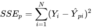
- is the error sum of squares for the model with p regressors,
- Ypi is the predicted value of the ith observation of Y from the p regressors,
- S2 is the estimation of residuals variance after regression on the complete set of k regressors and can be estimated by ,[1]
- and N is the sample size.

Alternative definition
[edit]Given a linear model such as:

where:
- are coefficients for predictor variables
- represents error


An alternate version of can also be defined as:[5]

where
- RSS is the residual sum of squares on a training set of data
- p is the number of predictors
- and refers to an estimate of the variance associated with each response in the linear model (estimated on a model containing all predictors)
Note that this version of the does not give equivalent values to the earlier version, but the model with the smallest from this definition will also be the same model with the smallest from the earlier definition.
Limitations
[edit]The criterion suffers from two main limitations[6]
- the approximation is only valid for large sample size;
- the ' cannot handle complex collections of models as in the variable selection (or feature selection) problem.[6]
Practical use
[edit]The statistic is often used as a stopping rule for various forms of stepwise regression. Mallows proposed the statistic as a criterion for selecting among many alternative subset regressions. Under a model not suffering from appreciable lack of fit (bias), has expectation nearly equal to p; otherwise the expectation is roughly P plus a positive bias term. Nevertheless, even though it has expectation greater than or equal to p, there is nothing to prevent Cp < p or even in extreme cases. It is suggested that one should choose a subset that has approaching p,[7] from above, for a list of subsets ordered by increasing p. In practice, the positive bias can be adjusted for by selecting a model from the ordered list of subsets, such that .


Since the sample-based statistic is an estimate of the MSPE, using for model selection does not completely guard against overfitting. For instance, it is possible that the selected model will be one in which the sample was a particularly severe underestimate of the MSPE.
Model selection statistics such as are generally not used blindly, but rather information about the field of application, the intended use of the model, and any known biases in the data are taken into account in the process of model selection.
See also
[edit]References
[edit]- ^ a b Mallows, C. L. (1973). "Some Comments on CP". Technometrics. 15 (4): 661–675. doi:10.2307/1267380. JSTOR 1267380.
- ^ Gilmour, Steven G. (1996). "The interpretation of Mallows's Cp-statistic". Journal of the Royal Statistical Society, Series D. 45 (1): 49–56. JSTOR 2348411.
- ^ Hirotugu Akaike (1973). "Information Theory and an Extension of the Maximum Likelihood Principle". Proceeding of the Second International Symposium on Information Theory: 267–281. Wikidata Q134962967.
- ^ Hirotugu Akaike (December 1974). "A New Look at the Statistical Model Identification". IEEE Transactions on Automatic Control. 19 (6): 716–723. doi:10.1109/TAC.1974.1100705. ISSN 0018-9286. PMID 40793584. Zbl 0314.62039. Wikidata Q26778401.
- ^ Gareth James; Daniela Witten; Trevor Hastie; Robert Tibshirani (2013). An Introduction to Statistical Learning: with Applications in R. Springer Texts in Statistics. Springer Science+Business Media. doi:10.1007/978-1-4614-7138-7. ISBN 978-1-4614-7137-0. LCCN 2013936251. OCLC 1004563473. OL 26184759M. Zbl 1281.62147. Wikidata Q21473973.
- ^ a b Giraud, C. (2015), Introduction to high-dimensional statistics, Chapman & Hall/CRC, ISBN 9781482237948
- ^ Daniel, C.; Wood, F. (1980). Fitting Equations to Data (Rev. ed.). New York: Wiley & Sons, Inc.
Further reading
[edit]- Chow, Gregory C. (1983). Econometrics. New York: McGraw-Hill. pp. 291–293. ISBN 978-0-07-010847-9.
- Hocking, R. R. (1976). "The analysis and selection of variables in linear regression". Biometrics. 32 (1): 1–50. CiteSeerX 10.1.1.472.4742. doi:10.2307/2529336. JSTOR 2529336.
- Judge, George G.; Griffiths, William E.; Hill, R. Carter; Lee, Tsoung-Chao (1980). The Theory and Practice of Econometrics. New York: Wiley. pp. 417–423. ISBN 978-0-471-05938-7.
Grokipedia
Mallows's Cp
View on GrokipediaBackground
Linear Regression Context
In ordinary least squares (OLS) regression, the model posits a linear relationship between a response vector and a design matrix of predictors, expressed as , where is the vector of unknown coefficients and is the error term typically assumed to follow a multivariate normal distribution with mean zero, constant variance , and identity covariance matrix .[3] The OLS estimator minimizes the sum of squared residuals to obtain , providing unbiased and efficient estimates under the model's assumptions.[3] The validity of OLS inferences relies on four key assumptions: linearity, which requires the conditional expectation to hold; independence, ensuring observations are independent such that residuals are uncorrelated; homoscedasticity, meaning the error variance is constant across all levels of the predictors; and normality, where errors are normally distributed for exact finite-sample inference, though this is less critical for large samples due to the central limit theorem.[4] Violations of these assumptions, such as nonlinearity or heteroscedasticity, can lead to biased estimates, inefficient predictions, or invalid hypothesis tests.[5] In multiple linear regression, incorporating numerous predictors allows for capturing complex relationships but introduces the risk of overfitting, where the full model including all predictors fits the training data excessively well at the expense of generalizability.[6] Submodels, which select a subset of predictors, aim to balance fit and parsimony, reducing variance and mitigating overfitting by excluding irrelevant variables that inflate estimation error on new data.[6] This tradeoff is particularly acute when approaches or exceeds the sample size , as the full model may capture noise rather than signal.[6] The development of subset selection methods in linear regression gained prominence in the 1960s and 1970s, coinciding with advances in computational power that made exhaustive searches feasible beyond manual calculations.[7] Prior to the 1970s, computing all subsets was prohibitively expensive, limiting analyses to simple or stepwise approaches, but improved algorithms and hardware enabled more systematic exploration of model spaces.[7] This era marked a shift toward automated variable selection to handle growing datasets in fields like econometrics and environmental modeling.Model Selection Challenges
In multiple linear regression, selecting an appropriate subset of predictor variables from a larger set poses significant challenges, as the goal is to identify a model that accurately captures the underlying relationships in the data while avoiding excessive complexity or oversimplification. This process is complicated by the need to balance the desire for a good fit to the observed data with the risk of poor performance on new, unseen data, particularly under the standard assumptions of linearity, independence, and homoscedasticity in residuals.[8] One primary issue is overfitting, where including too many predictors results in a model that fits the training data excessively well, achieving low residual error on the sample but failing to generalize to independent data due to capturing noise rather than true signal. Conversely, underfitting arises when relevant predictors are excluded, leading to a model that is too simplistic and exhibits high bias by systematically missing key patterns in the data, thereby producing consistently poor predictions across both training and test sets.[8] These risks highlight the delicate nature of subset selection, where the choice of predictors directly impacts the model's reliability for inference and prediction. At the heart of these challenges lies the bias-variance tradeoff, a fundamental principle in model selection that quantifies how increasing model complexity reduces bias (systematic error from model misspecification) but increases variance (sensitivity to fluctuations in the training data), often leading to an optimal complexity level that minimizes overall prediction error. In linear regression contexts, this tradeoff necessitates criteria that penalize excessive parameters to prevent variance-dominated models, ensuring the selected subset provides a stable estimate of the true regression surface without unnecessary variability.[9] A further complication is the computational explosion inherent in exhaustive subset selection, as evaluating all possible combinations of p predictors requires fitting 2p distinct models, rendering the approach infeasible for even moderately large p (e.g., beyond 20-30 variables) due to the exponential growth in time and resources.[10] This scalability issue has historically driven the development of heuristic alternatives, though it underscores the need for efficient, principled methods to navigate the vast search space without exhaustive enumeration. Early approaches to address these problems, such as stepwise regression (including forward, backward, and bidirectional variants), attempt to approximate optimal subsets through greedy algorithms that iteratively add or remove predictors based on statistical criteria like p-values or information measures.[11] However, these methods suffer from inherent limitations, including their greedy nature, which commits to local decisions without reconsidering global optimality, potentially leading to suboptimal models, biased parameter estimates, and inconsistencies across different algorithmic implementations.[11] Additionally, stepwise procedures can inflate Type I errors by repeatedly testing variables on the same dataset, exacerbating overfitting risks in high-dimensional settings.[12]Mathematical Formulation
Original Definition
Mallows's statistic was introduced by Colin L. Mallows in 1973 as a criterion for selecting subset regression models in linear regression. The original formulation defines for a submodel with parameters (including the intercept) asKey Properties and Derivation
Mallows's statistic is derived as an estimator of the mean squared error of prediction (MSEP) for a linear regression model with parameters, where MSEP quantifies the expected prediction error for new observations. Specifically, for a new response at covariates , the MSEP is given byAlternative Expressions
Residual Sum of Squares Form
An equivalent formulation of Mallows's expresses the criterion directly in terms of the residual sum of squares (RSS) from the candidate subset model and the full model, eliminating the need for an explicit estimate of the error variance beyond what is inherent in the RSS values. Specifically, for a subset model with predictors (totaling parameters including the intercept), the RSS form is given byRelationship to Prediction Error
Mallows's criterion is closely connected to the predicted residual sum of squares (PRESS) statistic, which serves as a direct measure of a model's predictive accuracy through leave-one-out cross-validation. The PRESS is defined as the sum of squared prediction errors obtained by omitting each observation in turn and predicting it using the model fitted to the remaining data:Computation and Estimation
Step-by-Step Calculation
To compute Mallows's statistic for model selection in linear regression, begin by fitting the full model that includes all candidate predictors using ordinary least squares (OLS). Let denote the number of observations, and let the full model have parameters (including the intercept). Compute the residual sum of squares for this full model, denoted , and estimate the error variance as . This plug-in estimate accounts for the uncertainty in the true variance , providing a stable denominator for subsequent calculations across submodels.[13] Next, for each candidate submodel with effective parameters (including the intercept), fit the model via OLS on the selected predictors while setting coefficients for excluded variables to zero. Obtain the residual sum of squares for this submodel, where and are the fitted values. The parameter count reflects the dimensionality of the submodel, typically ranging from 1 (intercept only) to (full model).[13] Finally, substitute these values into the formula:Illustrative Example
Consider a hypothetical dataset with observations and 3 candidate predictors (), so the full model has parameters (including intercept). Suppose fitting the full model yields , giving . For submodel 1 using only (), OLS fitting gives . Then,Software Implementation
Mallows's is commonly implemented in statistical software for subset selection in linear regression, leveraging exhaustive or heuristic searches to evaluate models based on the criterion. In R, theleaps package provides an efficient branch-and-bound algorithm for best subset regression, computing values across possible subsets.[16] For example, the regsubsets function can be used as follows:
library(leaps)
model <- regsubsets(x = predictors, y = response, nvmax = 10, method = "exhaustive")
cp_values <- summary(model)$cp
plot(cp_values, main = "Mallows's Cp by Number of Predictors")
leaps in scikit-learn or statsmodels for exhaustive subset selection with , due to the combinatorial explosion in high dimensions; instead, custom implementations combine itertools.combinations for subset enumeration with statsmodels.OLS for fitting and calculation.[17] A representative custom function might iterate over subsets up to a specified size, compute the residual sum of squares (RSS), and derive , where is the mean squared error from the full model:
import itertools
import statsmodels.api as sm
import numpy as np

def mallows_cp(X, y, max_features=5):
    full_model = sm.OLS(y, sm.add_constant(X)).fit()
    s2 = full_model.mse_resid
    n, p = X.shape
    best_cp = float('inf')
    for k in range(1, min(max_features + 1, p + 1)):
        for combo in itertools.combinations(range(p), k):
            X_subset = X[list(combo)]
            model = sm.OLS(y, sm.add_constant(X_subset)).fit()
            rss = model.ssr
            cp = (rss / s2) + 2 * (k + 1) - n
            if cp < best_cp:
                best_cp = cp
    return best_cp
SELECTION=CP option in the MODEL statement performs forward, backward, or stepwise selection minimizing , outputting selected models and statistics. For instance:
proc reg data=mydata;
   model response = var1 var2 var3 / selection=cp;
run;
regress but can be computed post-estimation using the user-contributed rsquare command, which calculates alongside other criteria after fitting models.
Post-2020 developments have enhanced workflow integration and scalability. In R's tidymodels ecosystem, the broom package tidies outputs from leaps::regsubsets, enabling seamless piping with dplyr and ggplot2 for automated model selection and visualization within machine learning pipelines.[18] For high-dimensional data where , exact computation becomes infeasible, and approximations via penalized regression in the glmnet package use LASSO paths to mimic subset selection, with analogs like generalized cross-validation (GCV) for tuning. The exact exhaustive search for has computational complexity in the naive case, due to subsets and least squares fits each, though optimized algorithms like branch-and-bound reduce the constant factors but retain exponential dependence on .[19]