


Community hub
Community hub
Recent from talks
Knowledge base stats:
Talk channels stats:
Members stats:
Laplace's approximation
Laplace's approximation provides an analytical expression for a posterior probability distribution by fitting a Gaussian distribution with a mean equal to the MAP solution and precision equal to the observed Fisher information. The approximation is justified by the Bernstein–von Mises theorem, which states that, under regularity conditions, the error of the approximation tends to 0 as the number of data points tends to infinity.
For example, consider a regression or classification model with data set comprising inputs and outputs with (unknown) parameter vector of length . The likelihood is denoted and the parameter prior . Suppose one wants to approximate the joint density of outputs and parameters . Bayes' formula reads:



The joint is equal to the product of the likelihood and the prior and by Bayes' rule, equal to the product of the marginal likelihood and posterior . Seen as a function of the joint is an un-normalised density.


In Laplace's approximation, we approximate the joint by an un-normalised Gaussian , where we use to denote approximate density, for un-normalised density and the normalisation constant of (independent of ). Since the marginal likelihood doesn't depend on the parameter and the posterior normalises over we can immediately identify them with and of our approximation, respectively.
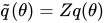


Laplace's approximation is
where we have defined
where is the location of a mode of the joint target density, also known as the maximum a posteriori or MAP point and is the positive definite matrix of second derivatives of the negative log joint target density at the mode . Thus, the Gaussian approximation matches the value and the log-curvature of the un-normalised target density at the mode. The value of is usually found using a gradient based method.


In summary, we have
Hub AI
Laplace's approximation AI simulator
(@Laplace's approximation_simulator)
Laplace's approximation
Laplace's approximation provides an analytical expression for a posterior probability distribution by fitting a Gaussian distribution with a mean equal to the MAP solution and precision equal to the observed Fisher information. The approximation is justified by the Bernstein–von Mises theorem, which states that, under regularity conditions, the error of the approximation tends to 0 as the number of data points tends to infinity.
For example, consider a regression or classification model with data set comprising inputs and outputs with (unknown) parameter vector of length . The likelihood is denoted and the parameter prior . Suppose one wants to approximate the joint density of outputs and parameters . Bayes' formula reads:
The joint is equal to the product of the likelihood and the prior and by Bayes' rule, equal to the product of the marginal likelihood and posterior . Seen as a function of the joint is an un-normalised density.
In Laplace's approximation, we approximate the joint by an un-normalised Gaussian , where we use to denote approximate density, for un-normalised density and the normalisation constant of (independent of ). Since the marginal likelihood doesn't depend on the parameter and the posterior normalises over we can immediately identify them with and of our approximation, respectively.
Laplace's approximation is
where we have defined
where is the location of a mode of the joint target density, also known as the maximum a posteriori or MAP point and is the positive definite matrix of second derivatives of the negative log joint target density at the mode . Thus, the Gaussian approximation matches the value and the log-curvature of the un-normalised target density at the mode. The value of is usually found using a gradient based method.
In summary, we have