Hubbry Logo
search
logo
1648731

Spatial multiplexing

logo
Community Hub0 Subscribers
Read side by side
from Wikipedia
Spatial multiplexing
2xSMX or STC+2xMRC

Spatial multiplexing or space-division multiplexing (SM, SDM or SMX) is a multiplexing technique in MIMO wireless communication, fiber-optic communication and other communications technologies used to transmit independent channels separated in space.

Fiber-optic communication

[edit]

In fiber-optic communication SDM refers to the usage of the transverse dimension of the fiber to separate the channels.

Techniques

[edit]

Multi-core fiber (MCF)

[edit]

Multi-core fibers are designed with more than a single core. Different types of MCFs exist, of which “Uncoupled MCF” is the most common, in which each core is treated as an independent optical path. The main limitation of these systems is the presence of inter-core crosstalk. In recent times, different splicing techniques, and coupling methods have been proposed and demonstrated, and despite many of the component technologies still being in the development stage, MCF systems already present the capability for huge transmission capacity.[citation needed]

Recently, some developed component technologies for multicore optical fiber have been demonstrated, such as three-dimensional Y-splitters between different multicore fibers,[1] a universal interconnection among the same fiber cores,[2] and a device for fast swapping and interchange of wavelength-division multiplexed data among cores of multicore optical fiber.[3]

Multi-mode fibers (MMF) and Few-mode fibers (FMF)

[edit]

Multi-mode fibers have a larger core that allows the propagation of multiple cylindrical transverse modes (Also referred as linearly polarized modes), in contrast to a single mode fiber (SMF) that only supports the fundamental mode. Each transverse mode is spatially orthogonal, and allows for the propagation in both orthogonal polarization.

Typical MMF are currently not viable for SDM, as the high mode count results in unmanageable levels of modal coupling and dispersion. The utilization of few-mode fibers, which are MMFs with a core size designed specially to allow a low count of spatial modes, is currently under consideration.

Due to physical imperfections, the modes exchange power and are experience different effective refractive indexes as they propagate through the fiber.[4] The power exchange results in modal coupling, and this effect is known to reduce the achievable capacity of the fiber,[5] if the modes experience unequal gain or attenuation. Therefore, if not compensated, the capacity increase is not linear to the mode count. The effective refractive index difference results in inter-symbolic interference, resulting from delay spread.[6]

Mode multiplexers consist of photonic lanterns, multi-plane light conversion, and others.

Fiber bundles

[edit]

Bundled fibers are also considered a form of SDM.

Wireless communications
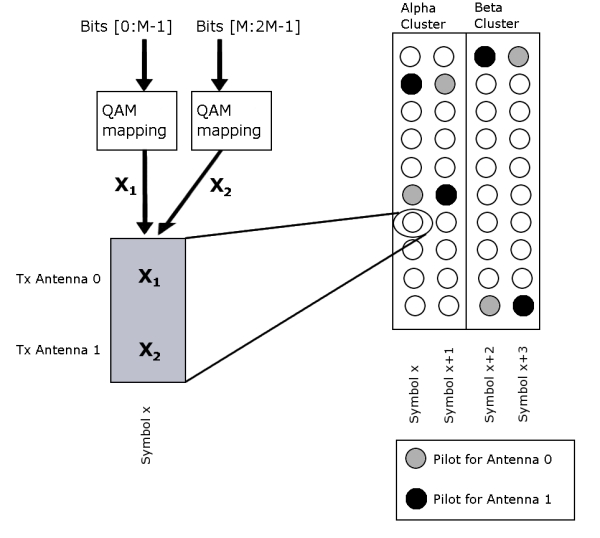
[edit]

If the transmitter is equipped with antennas and the receiver has antennas, the maximum spatial multiplexing order (the number of streams) is,

if a linear receiver is used. This means that streams can be transmitted in parallel, ideally leading to an increase of the spectral efficiency (the number of bits per second per Hz that can be transmitted over the wireless channel). The practical multiplexing gain can be limited by spatial correlation, which means that some of the parallel streams may have very weak channel gains.

Encoding

[edit]

Open-loop approach

[edit]

In an open-loop MIMO system with transmitter antennas and receiver antennas, the input-output relationship can be described as

where is the vector of transmitted symbols, are the vectors of received symbols and noise respectively and is the matrix of channel coefficients. An often encountered problem in open loop spatial multiplexing is to guard against instance of high channel correlation and strong power imbalances between the multiple streams. One such extension which is being considered for DVB-NGH systems is the so-called enhanced Spatial Multiplexing (eSM) scheme.

Closed-loop approach

[edit]

A closed-loop MIMO system utilizes Channel State Information (CSI) at the transmitter. In most cases, only partial CSI is available at the transmitter because of the limitations of the feedback channel. In a closed-loop MIMO system the input-output relationship with a closed-loop approach can be described as

where is the vector of transmitted symbols, are the vectors of received symbols and noise respectively, is the matrix of channel coefficients and is the linear precoding matrix.

A precoding matrix is used to precode the symbols in the vector to enhance the performance. The column dimension of can be selected smaller than which is useful if the system requires streams because of several reasons. Examples of the reasons are as follows: either the rank of the MIMO channel or the number of receiver antennas is smaller than the number of transmit antennas.

See also

[edit]

References

[edit]
Revisions and contributorsEdit on WikipediaRead on Wikipedia
from Grokipedia
Spatial multiplexing, also known as space-division multiplexing (SDM), is a multiplexing technique used in both wireless multiple-input multiple-output (MIMO) systems and optical fiber communications, enabling the simultaneous transmission of multiple independent data streams over the same frequency or wavelength by utilizing multiple spatial channels at both the transmitter and receiver ends.[1] This approach exploits the spatial dimension of the communication channel to achieve higher spectral efficiency and increased data throughput without requiring additional bandwidth or power.[2] The concept of spatial multiplexing originated in the early 1990s, with foundational work by Arogyaswami Paulraj and Thomas Kailath, who proposed using MIMO for spatial multiplexing in a 1993 patent that described transmitting independent signals via multiple antennas to enhance capacity in fading environments. This idea was further advanced by Gerard J. Foschini in 1996, who introduced the layered space-time architecture, demonstrating theoretically and experimentally how multiple antennas could support parallel data streams in rich scattering channels.[3] Bell Labs later developed the V-BLAST (Vertical Bell Laboratories Layered Space-Time) prototype in 1998, providing the first practical demonstration of spatial multiplexing with significant capacity gains. At its core, spatial multiplexing operates by encoding separate data streams onto different spatial channels, where the receiver uses channel state information to separate and decode these streams, often via techniques like singular value decomposition (SVD) that diagonalizes the channel matrix into parallel subchannels.[2] The achievable capacity scales linearly with the minimum of the number of transmit and receive channels (min(N_t, N_r)) in high signal-to-noise ratio (SNR) conditions, provided the channel has full rank due to sufficient multipath scattering or modal diversity.[1] Detection methods such as zero-forcing (ZF), minimum mean square error (MMSE), or successive interference cancellation (SIC) are commonly used to mitigate inter-stream interference, though they must balance performance against computational complexity.[1] Spatial multiplexing has become integral to modern communication standards, including Wi-Fi (IEEE 802.11n and later), LTE, and 5G NR in wireless systems, where it supports multi-user scenarios and massive MIMO configurations to deliver gigabit speeds and improved reliability in dense environments. In optical communications, it is employed in space-division multiplexing schemes using multi-core fibers, few-mode fibers, and fiber bundles to achieve higher data rates in long-haul transmission systems.[4] Its adoption has driven a fundamental shift in communication design, prioritizing multiplexing gains over traditional techniques in bandwidth-limited scenarios, while ongoing research addresses challenges like modal crosstalk and interference in next-generation systems.[5]

Fundamentals

Definition and principles

Spatial multiplexing, also known as space-division multiplexing (SDM), is a communication technique that exploits multiple parallel spatial channels to transmit independent data streams simultaneously, thereby increasing overall capacity without requiring additional bandwidth or transmit power.[6][4] This approach leverages the physical separation of signal paths—such as distinct antennas in wireless systems or separate cores and modes in optical fibers—to achieve orthogonality among channels, allowing for higher throughput in multipath-rich environments.[7] In contrast to time-division multiplexing (TDM), which allocates sequential time slots to different signals, frequency-division multiplexing (FDM), which divides the spectrum into non-overlapping bands, and polarization-division multiplexing (PDM), which uses orthogonal polarization states, SDM relies on spatial dimensions for separation rather than temporal, spectral, or polarization degrees of freedom.[6][8] For instance, in wireless communications, spatial paths arise from multipath propagation, where signals reflect off surroundings to create resolvable paths between antennas, while in optical communications, modal dispersion— the spreading of light pulses due to varying propagation speeds across different fiber modes—provides the necessary spatial diversity at an introductory level.[4] The basic operational principle involves a transmitter encoding distinct data streams onto separate spatial paths, such as by precoding signals for transmission across multiple antennas or modes, followed by a receiver that employs signal processing techniques—like matrix inversion or singular value decomposition—to demultiplex and recover the original streams with minimal interference.[6][4] This process assumes channel state information is available to enable effective separation, ensuring the signals remain distinguishable despite potential crosstalk. A key benefit of spatial multiplexing is its potential for linear capacity scaling with the number of spatial channels; for example, employing N independent channels can theoretically multiply the data rate by up to N compared to a single-channel system, addressing capacity limitations in high-demand networks.[7] In practice, this is exemplified in wireless systems through multiple-input multiple-output (MIMO) configurations and in optics via multi-core fibers, where multiple parallel cores serve as distinct spatial paths.[8]

Mathematical formulation

The mathematical formulation of spatial multiplexing begins with the standard linear signal model for a multiple-input multiple-output (MIMO) system. Consider a system equipped with NtN_t transmit antennas and NrN_r receive antennas. The received signal vector yCNr\mathbf{y} \in \mathbb{C}^{N_r} is given by y=Hx+n\mathbf{y} = \mathbf{H} \mathbf{x} + \mathbf{n}, where xCNt\mathbf{x} \in \mathbb{C}^{N_t} is the transmitted signal vector, HCNr×Nt\mathbf{H} \in \mathbb{C}^{N_r \times N_t} is the channel matrix describing the propagation between transmit and receive antennas, and nCNr\mathbf{n} \in \mathbb{C}^{N_r} is additive white Gaussian noise (AWGN) with zero mean and covariance σ2INr\sigma^2 \mathbf{I}_{N_r}.[9] The capacity of this MIMO channel under spatial multiplexing, assuming full channel state information (CSI) at the receiver and no CSI at the transmitter, is achieved by treating the channel as a set of parallel subchannels. With an average transmit power constraint PP, the capacity CC is expressed as
C=log2det(INr+ρNtHHH), C = \log_2 \det \left( \mathbf{I}_{N_r} + \frac{\rho}{N_t} \mathbf{H} \mathbf{H}^H \right),
where ρ=P/σ2\rho = P / \sigma^2 is the signal-to-noise ratio (SNR), INr\mathbf{I}_{N_r} is the Nr×NrN_r \times N_r identity matrix, and HH\mathbf{H}^H denotes the Hermitian transpose of H\mathbf{H}. This formula quantifies the multiplexing gain, which grows linearly with min(Nt,Nr)\min(N_t, N_r) at high SNR, enabling the transmission of multiple independent data streams simultaneously.[9] For fading channels where H\mathbf{H} varies randomly over time or frequency, the ergodic capacity replaces the deterministic capacity, representing the long-term average rate. The ergodic capacity is the expected value C=E[log2det(INr+ρNtHHH)]C = \mathbb{E} \left[ \log_2 \det \left( \mathbf{I}_{N_r} + \frac{\rho}{N_t} \mathbf{H} \mathbf{H}^H \right) \right], taken over the distribution of H\mathbf{H} (typically Rayleigh fading, where entries of H\mathbf{H} are independent complex Gaussian). This measures the average achievable rate under spatial multiplexing in time-varying environments.[9] The derivation of the capacity formula stems from information theory, specifically the maximization of mutual information I(x;y)I(\mathbf{x}; \mathbf{y}) between input x\mathbf{x} and output y\mathbf{y} under the power constraint, with Gaussian signaling being optimal. The singular value decomposition (SVD) of the channel matrix, H=UΣVH\mathbf{H} = \mathbf{U} \boldsymbol{\Sigma} \mathbf{V}^H, decomposes the MIMO channel into min(Nt,Nr)\min(N_t, N_r) parallel non-interacting subchannels with gains given by the singular values in the diagonal matrix Σ\boldsymbol{\Sigma}. The capacity then becomes the sum of the capacities of these subchannels, i=1min(Nt,Nr)log2(1+λiγi)\sum_{i=1}^{\min(N_t, N_r)} \log_2 (1 + \lambda_i \gamma_i), where λi\lambda_i are the singular values and γi\gamma_i are the effective SNRs after power allocation.[9] To achieve the optimal rate, water-filling power allocation is applied across the eigenmodes (subchannels). The power pip_i allocated to the ii-th subchannel is pi=max(0,μ1/λi2)p_i = \max(0, \mu - 1/\lambda_i^2), where μ\mu is chosen to satisfy the total power constraint pi=P\sum p_i = P. This uneven distribution favors stronger subchannels (larger λi\lambda_i), pouring more power where the noise inverse is higher, thereby maximizing the overall capacity.[9] In optical communications, spatial multiplexing generalizes to similar matrix-based models, where the channel matrix H\mathbf{H} captures mode coupling or crosstalk between spatial channels (e.g., cores or modes) in multi-core or multi-mode fibers, with the received signal following an analogous linear form y=Hx+n\mathbf{y} = \mathbf{H} \mathbf{x} + \mathbf{n}. The capacity expressions adapt accordingly, though noise may include additional optical impairments like amplifier noise, while preserving the MIMO-like structure for multiplexing gains.[10]

Historical development

In wireless communications

The origins of spatial multiplexing in wireless communications trace back to early theoretical work in the 1990s, when Arogyaswami Paulraj and Thomas Kailath filed a patent in 1992 that was granted in 1994, describing a method to increase capacity in wireless systems by using arrays of multiple transmitting and receiving antennas to exploit multipath propagation as a resource rather than an impairment.[11] This approach, known as spatial multiplexing, enabled the transmission of independent data streams over the same frequency band, effectively creating parallel channels in rich-scattering environments.[12] Key advancements came through seminal publications that formalized the technique and quantified its potential. In 1996, Gerard Foschini at Bell Labs proposed a layered space-time architecture for spatial multiplexing in fading channels using multi-element antennas, laying the groundwork for practical MIMO systems by demonstrating how multiple streams could be decoded successively.[3] Building on this, Foschini and Michael Gans published in 1998 on the limits of wireless communications in fading environments with multiple antennas, showing that such systems could achieve capacities far exceeding traditional single-antenna bounds by leveraging multipath.[13] Concurrently, Emre Telatar's 1999 analysis (circulated internally earlier) derived the ergodic capacity of MIMO channels, establishing that under rich scattering, capacity scales linearly with the minimum of the number of transmit and receive antennas, marking spatial multiplexing as a breakthrough for surpassing the Shannon limit in wireless.[9] A pivotal milestone was the first experimental demonstration of spatial multiplexing by Lucent Technologies' Bell Labs in 1998, using a V-BLAST prototype that demonstrated spectral efficiencies of 20-40 bps/Hz in an indoor rich-scattering environment at short range (tens of meters), validating the theoretical gains in real-world settings.[14] This demo highlighted the technique's ability to overcome the conventional Shannon capacity limit for single-antenna systems by turning multipath-rich urban and indoor environments—characterized by numerous scattering paths—into an asset for supporting multiple orthogonal streams without interference.[15] The transition to standards began in the 2000s with integration into 3G systems; specifically, MIMO spatial multiplexing was standardized for HSDPA in 3GPP Release 7 (2007), enabling up to 28.8 Mbps peak downlink rates through 2x2 configurations.[16] In 4G LTE (3GPP Release 8, commercialized around 2009), spatial multiplexing supported up to 8x8 MIMO configurations, boosting spectral efficiency and peak rates to over 300 Mbps in advanced deployments.[17] By 5G NR (3GPP Release 15, 2018), massive MIMO extended spatial multiplexing to 64 or more antennas, facilitating multi-user scenarios and capacities exceeding 10 Gbps in dense urban settings with abundant multipath.[18]

In optical communications

In the post-2000s era, the rapid growth of internet traffic led to a "capacity crunch" in optical networks, primarily due to the nonlinear Shannon limit imposed by fiber nonlinearities in single-mode fibers (SMF), which constrained further scaling of wavelength-division multiplexing (WDM) capacities.[19] This limitation prompted the proposal of space-division multiplexing (SDM) around 2010 as a strategy to spatially reuse existing WDM capacities by introducing multiple parallel transmission paths within a single fiber.[7] Key milestones in optical SDM began with early prototypes and transmission experiments. In 2009–2010, OFS Laboratories developed initial multi-core fiber (MCF) prototypes featuring seven cores arranged in a hexagonal pattern, demonstrating low crosstalk suitable for passive optical networks.[20] This was followed in 2011 by the National Institute of Information and Communications Technology (NICT) in Japan achieving the first high-capacity MCF transmission, with 109 Tb/s over 16.8 km using seven cores, 97 WDM channels, and polarization-division multiplexing (PDM) QPSK signals.[21] Mode-division multiplexing (MDM) demonstrations emerged around the same period, with 2011–2012 experiments using few-mode fibers (FMF) to transmit multiple spatial modes over distances up to 96 km, leveraging coherent 6×6 MIMO processing for six spatial and polarization modes at 40 Gb/s each.[22] Standardization efforts for SDM in optical communications commenced with ITU-T studies in 2020, focusing on integrating SDM with existing WDM infrastructure.[23] By 2015, advancements enabled the integration of SDM with coherent detection techniques for long-haul applications, allowing robust signal recovery in MCF and FMF systems over thousands of kilometers through digital signal processing to mitigate modal crosstalk and dispersion.[24] Pioneering contributions also came from Bell Laboratories, which in 2013 advanced SDM system designs incorporating MIMO techniques to address nonlinear impairments in multi-core and multi-mode fibers.[25] European initiatives, such as the EU-funded INSPACE project in the 2010s, further drove SDM networking solutions, emphasizing spatial-spectral flexibility for ultra-high-capacity transport. The evolution of SDM in telecom marked a shift from early 1980s fiber bundles, primarily used for imaging applications like endoscopy where loose arrays of fibers transmitted light without multiplexing for data, to integrated fibers in the 2010s revival for telecommunications.[26] This transition enabled scalable, low-crosstalk spatial channels in MCF and FMF, overcoming the bulkiness and inefficiency of bundles for high-speed, long-haul data transmission. Recent advancements include NICT's 2024 demonstration of 22.9 Pb/s over 52.4 km using a 4-core fiber, pushing SDM capacities further.[27][7]

Applications in fiber-optic communications

Multi-core fibers

Multi-core fibers (MCFs) integrate multiple isolated cores within a single common cladding to enable spatial division multiplexing (SDM) in optical fiber communications, typically accommodating 7 to 19 cores arranged in configurations such as hexagonal lattices for efficient packing and minimal interference.[28] These cores function as parallel waveguides, each supporting independent light propagation while sharing the surrounding cladding to maintain a standard fiber diameter of around 125 μm.[29] MCF designs are broadly classified into uncoupled-core variants, which prioritize low inter-core interaction to treat each core as a distinct spatial channel, and coupled-core variants, which permit controlled coupling to leverage mode mixing for enhanced capacity in certain scenarios.[30] In transmission systems, each core of an MCF carries a separate wavelength-division multiplexed (WDM) signal, allowing the aggregate data capacity to scale directly with the number of cores and thereby overcoming the nonlinear capacity limits of single-core fibers.[31] For example, in 2025, a 19-core MCF enabled 1.02 Pb/s transmission over 1,808 km by multiplexing C+L band signals across the cores.[32] Fabrication of MCFs predominantly relies on the stack-and-draw technique, where multiple core rods are stacked into a preform assembly and thermally drawn into a continuous fiber, enabling precise control over core positioning and refractive index profiles.[33] Early challenges in achieving core uniformity, such as variations in diameter and spacing that could induce losses or crosstalk, have been addressed through 2020s advancements in modified chemical vapor deposition and automated stacking processes, resulting in improved yield and consistency for commercial-scale production.[34][35] Managing inter-core coupling is critical in MCFs to ensure signal integrity, with uncoupled designs targeting inter-core crosstalk (XT) levels below -30 dB/km to minimize power transfer between adjacent cores over transmission distances.[36] This is often achieved through trench-assisted cladding structures, which incorporate low-index trenches surrounding each core to increase modal confinement and suppress evanescent field overlap, thereby reducing XT without significantly raising bending losses.[37] In advanced implementations, such as 4-core MCFs, XT has been lowered to below -60 dB/100 km alongside ultra-low attenuation of 0.155 dB/km.[38] MCFs find prominent applications in short-reach interconnects for data centers, where their high spatial density supports massive parallelism in intra- and inter-rack communications without expanding cable footprints.[39] For instance, 12-core MCF links have been integrated into 2023 hyper-scale data center networks to deliver enhanced throughput for AI-driven workloads, enabling denser fiber routing and reduced latency in environments demanding terabit-scale bandwidth over distances up to several kilometers.[40]

Multi-mode and few-mode fibers

Few-mode fibers (FMFs) are specialized optical fibers designed to support a limited number of guided modes, typically ranging from 2 to 10 linearly polarized (LP) modes, such as LP01 (the fundamental mode) and LP11, enabling controlled propagation for mode-division multiplexing (MDM) in spatial division multiplexing (SDM) systems.[41][42] In contrast, multi-mode fibers (MMFs) support over 100 modes, leading to significant modal dispersion that limits their use to shorter distances.[41] FMFs leverage these orthogonal spatial modes as independent channels, often combined with wavelength-division multiplexing (WDM) to increase overall capacity, while requiring precise mode control to minimize intermodal coupling.[42] Mode-division multiplexing (MDM) in photonic systems, particularly when combined with WDM, significantly increases channel density by supporting multiple spatial modes per wavelength. For example, systems can achieve more than 4 modes per wavelength across 32-64 wavelengths, enabling densities exceeding 37 Tbps/cm².[43] This hybrid approach multiplies the effective channel density by a factor of 4-8 through the use of mode converters such as subwavelength gratings or microring resonators (MRR).[44][45] Such advancements facilitate higher computation rates, exceeding 500 Gops, in photonic integrated circuits without requiring an increase in chip size.[46] Multiplexing in FMFs and MMFs involves launching and detecting specific modes using devices like spatial light modulators (SLMs) for programmable wavefront shaping or photonic lanterns for efficient mode conversion from single-mode inputs.[47] At the receiver, multiple-input multiple-output (MIMO) digital signal processing (DSP) is essential for demultiplexing coupled modes, compensating for modal crosstalk and differential group delay (DGD) that arises from varying group velocities among modes.[48] DGD compensation, often achieved through adaptive DSP algorithms or fiber design optimizations, is critical to maintain signal integrity over long distances.[49] Performance demonstrations highlight FMF's potential for long-haul transmission; for instance, a 2023 experiment achieved 10 spatial modes over 1300 km using a 6-LP graded-index FMF with MIMO DSP.[50] For short-haul applications, graded-index MMFs, such as those meeting OM4 or OM5 standards, support data rates like 100 Gb/s over 100 m, benefiting from reduced modal dispersion compared to step-index designs.[51][52] Compared to multi-core fibers (MCFs), FMFs offer higher integration density by propagating multiple modes within a single core while adhering to the standard 125 μm cladding diameter, allowing scalability to up to 100 modes without increasing fiber size.[53] This compactness facilitates easier splicing and deployment, with potential applications in long-haul systems including submarine cables as part of ongoing SDM commercialization efforts as of 2025.[54]

Fiber bundles

Fiber bundles represent a straightforward implementation of spatial division multiplexing (SDM) by aggregating multiple individual optical fibers to parallelize data transmission channels. These bundles typically consist of single-mode fibers (SMFs) or multimode fibers (MMFs) arranged in parallel, enabling additive capacity scaling without the need for advanced modal or core integration. In SDM applications, fiber bundles serve as a basic aggregation method, particularly suited for short-reach or non-telecommunications scenarios where simplicity outweighs efficiency concerns.[55] Coherent fiber bundles maintain a fixed spatial arrangement of fibers from input to output ends, achieved by fusing or epoxy-bonding the fiber ends to preserve relative positions, which is essential for applications requiring image preservation. In contrast, incoherent bundles feature a random mapping between input and output fibers, prioritizing uniform light distribution over spatial fidelity. For SDM, both configurations can be employed, with SMF bundles favoring low-loss, long-distance parallel transmission and MMF bundles supporting higher modal diversity in shorter links. Fused ends in coherent bundles minimize misalignment but introduce coupling challenges at interfaces.[56][57][55] Early applications of fiber bundles emerged in medical imaging, particularly endoscopes, where coherent bundles transmitted high-resolution images from the 1980s onward. For instance, in 1982, techniques using fiber bundles enabled ultra-magnifying observation of colon mucosa, marking a key advancement in flexible endoscopy. In telecommunications, fiber bundles underpin low-speed parallel optics, such as 12-fiber MPO connectors, which facilitate 400 Gb/s Ethernet over parallel single-mode or multimode fibers up to 500 m. These connectors aggregate four 100 Gb/s lanes, supporting standards like IEEE 802.3bs for data center interconnects.[58][59] Despite their simplicity, fiber bundles suffer from significant limitations in SDM systems, including high insertion losses at fiber interfaces, often around 1.3 dB due to edge-coupling in fan-in/fan-out devices. Unlike multi-core fibers (MCFs), which integrate multiple channels monolithically within a single cladding for compact spatial efficiency, bundles lack such integration, resulting in bulkier cables and linearly scaling equipment costs—estimated at $20,000/km for deployment. This discrete nature also precludes benefits like reduced crosstalk management through coupled-core designs.[60][29] In modern prototypes, fiber bundles have been explored for orbital angular momentum (OAM) multiplexing, where bundles interface with glass chips to enable reversible OAM mode processing for enhanced channel capacity. Experiments in the 2020s have demonstrated OAM demultiplexing via fiber-bundle-coupled waveguides, achieving low-crosstalk handling of multiple OAM states in short-reach setups. Capacity in fiber bundles remains strictly additive per fiber, for example, aggregating 100 SMFs each supporting up to 100 Tb/s with WDM could yield 10 Pb/s total, though the resulting bulky form factor limits practicality for high-density deployments.[61]

Applications in wireless communications

MIMO systems

Multiple-input multiple-output (MIMO) systems form the cornerstone of spatial multiplexing in wireless communications, employing arrays of NtN_t transmit antennas at the base station and NrN_r receive antennas at the user equipment to simultaneously transmit multiple independent data streams over the same frequency band. This configuration exploits the spatial dimension of the wireless channel to achieve higher data rates without additional bandwidth or power, with the number of supported spatial streams limited by min(Nt,Nr)\min(N_t, N_r). In single-user MIMO (SU-MIMO), all streams are directed to a single user, maximizing throughput for that device by leveraging channel state information (CSI) to separate streams at the receiver.[62][63] In contrast, multi-user MIMO (MU-MIMO) serves multiple users concurrently by precoding streams to mitigate inter-user interference, enabling spatial multiplexing across users in downlink scenarios.[64] Integration of MIMO into cellular standards has progressively enhanced spatial multiplexing capabilities. In 4G LTE-Advanced, as defined by 3GPP Release 10, downlink spatial multiplexing supports up to 8 layers (streams) with configurations like 8x8 MIMO, allowing peak data rates of up to approximately 800 Mbps in 20 MHz bandwidth under ideal conditions.[65][66] For 5G New Radio (NR), 3GPP Release 15 and beyond incorporate massive MIMO with antenna arrays up to 256 elements, particularly in millimeter-wave (mmWave) bands above 24 GHz, where beamforming narrows beams to combat path loss while multiplexing dozens of streams. In 5G-Advanced (Release 18), enhancements include support for up to 4-layer uplink MIMO and refined CSI reporting to further improve spatial multiplexing performance.[67][68] Wireless channels in MIMO systems are commonly modeled as Rayleigh fading, where the channel matrix entries are independent complex Gaussian random variables, capturing the effects of multipath propagation without a dominant line-of-sight component. This model underpins the diversity-multiplexing tradeoff (DMT) curve, which characterizes the optimal balance between achieving high multiplexing gain (additional degrees of freedom for rate) and diversity gain (reliability against fading), as derived for high signal-to-noise ratio (SNR) regimes; for an Nt×NrN_t \times N_r system, the curve reveals that maximum multiplexing gain of min(Nt,Nr)\min(N_t, N_r) is attainable only at zero diversity, trading off for higher outage reliability at lower rates.[69] Hardware implementations of massive MIMO (mMIMO), with 100 or more antennas per base station, have scaled spatial multiplexing in real deployments. These systems use active antenna units (AAUs) integrating radio frequency chains and beamforming to support high-dimensional precoding, as seen in early 5G rollouts. For instance, Nokia's 2020 base station deployments with 64-antenna mMIMO configurations in urban macro cells achieved up to 10-fold throughput improvements over 4G LTE baselines, driven by enhanced spectral efficiency in multi-user scenarios.[70] At the receiver, spatial multiplexing streams are separated using linear decoding techniques such as zero-forcing (ZF) equalization, which inverts the channel matrix to null inter-stream interference at the cost of noise enhancement, or minimum mean square error (MMSE) equalization, which balances interference suppression with noise minimization for better performance in low-SNR conditions. ZF is computationally simpler and performs well in high-SNR rich-scattering environments, while MMSE approaches the optimal capacity more closely in practical Rayleigh fading channels.[71][72]

Open-loop techniques

Open-loop techniques in spatial multiplexing operate without channel state information (CSI) at the transmitter, relying instead on statistical knowledge of the channel to encode multiple data streams across spatial dimensions. These methods are particularly suited for scenarios with high mobility or fast-fading channels where feedback overhead would be impractical or unreliable. By avoiding the need for instantaneous CSI feedback, open-loop approaches simplify transmitter design and reduce latency, though they achieve multiplexing gains through predefined coding structures rather than adaptive optimization.[65] A foundational open-loop technique is space-time block coding (STBC), exemplified by the Alamouti scheme for two transmit antennas and one receive antenna (2x1 configuration). In this method, two symbols are transmitted over two time slots: in the first slot, symbol $ s_1 $ is sent from antenna 1 and $ s_2 $ from antenna 2; in the second slot, $ -s_2^* $ from antenna 1 and $ s_1^* $ from antenna 2, where $ ^* $ denotes complex conjugate. This orthogonal structure enables simple linear decoding at the receiver via maximal ratio combining, providing full diversity gain without CSI at the transmitter. The Alamouti code, introduced in 1998, achieves a coding rate of 1 while mitigating fading effects, making it robust for open-loop spatial multiplexing in early MIMO systems. For higher antenna configurations, cyclic delay diversity (CDD) extends open-loop multiplexing by applying cyclic shifts to the transmitted signals across antennas, effectively creating frequency-selective fading that enhances diversity. In CDD, the signal for each antenna is delayed by a fraction of the symbol period, turning the channel into a higher-rank equivalent for better separation of streams. This technique is particularly effective in orthogonal frequency-division multiplexing (OFDM) systems, as the delays introduce phase rotations across subcarriers, averaging out channel variations without requiring feedback. CDD supports up to four layers in multi-antenna setups and is standardized for scenarios where channel correlation is low.[73] Layered space-time coding, such as vertical Bell Laboratories Layered Space-Time (V-BLAST), represents another key open-loop algorithm for spatial multiplexing. V-BLAST divides the data stream into independent layers, each transmitted on a separate antenna, with the receiver employing successive interference cancellation (SIC) to detect and subtract layers sequentially. Ordering the layers by signal-to-noise ratio (SNR) during detection maximizes performance, achieving near-optimal capacity in rich-scattering environments. Developed in 1998, V-BLAST enables high spectral efficiency, with decoding complexity managed through ordered SIC, making it suitable for open-loop operation in dynamic channels. In terms of performance, open-loop techniques excel in fast-fading conditions, providing robustness against rapid channel changes. For instance, in 3GPP Long-Term Evolution (LTE) standards, open-loop spatial multiplexing uses predefined precoding matrices from codebooks—such as those based on CDD or rotation—to transmit up to four layers without CSI feedback, supporting single-user MIMO (SU-MIMO) in high-mobility scenarios like vehicular speeds up to 350 km/h. These methods yield multiplexing gains of up to 2x compared to single-input single-output (SISO) systems in typical urban environments, with throughput improvements demonstrated in field measurements showing doubled data rates at equivalent error rates.[74] Despite these advantages, open-loop techniques are suboptimal compared to closed-loop methods due to the lack of channel-specific adaptation, potentially limiting gains in correlated channels. To mitigate this, rotation-based precoding is often applied, where streams are rotated in the complex plane to average channel statistics and reduce inter-layer interference, enhancing robustness without feedback. This approach is widely adopted in 4G SU-MIMO for mobility, balancing simplicity and performance in real-world deployments.[75]

Closed-loop techniques

Closed-loop techniques in spatial multiplexing rely on channel state information (CSI) feedback from the receiver to the transmitter, enabling adaptive precoding that aligns transmission with the channel's spatial structure. The receiver estimates the CSI using pilot signals, quantizes it to manage feedback overhead, and transmits the quantized information back to the transmitter via a dedicated feedback channel. The transmitter then applies linear precoding based on this feedback to diagonalize the effective channel or suppress inter-user interference, thereby enhancing multiplexing gains in multi-antenna systems. This approach is particularly effective in slow-fading environments where channel variations are gradual, allowing reliable feedback without excessive latency. Key algorithms include singular value decomposition (SVD)-based precoding, which decomposes the channel matrix into parallel eigenmodes for optimal water-filling power allocation and spatial multiplexing across singular values. For multi-user MIMO (MU-MIMO), block diagonalization precoding eliminates inter-user interference by designing precoders orthogonal to other users' channel null spaces, approaching the sum capacity in high-SNR regimes with perfect CSI. In practical systems like LTE, limited feedback uses predefined codebooks where the receiver selects the best precoding matrix index (PMI), typically with 16 bits for up to four transmit antennas, enabling eigenmode transmission while constraining overhead. These codebooks are unitary matrices designed to minimize chordal distance to the ideal precoder, ensuring near-optimal performance with quantization error below 1 dB in typical scenarios.[76] In 5G New Radio (NR), CSI reporting is categorized into Type I and Type II for enhanced spatial multiplexing support. Type I provides coarse feedback with single-beam PMI for up to eight layers, suitable for single-user MIMO, while Type II offers finer granularity using multiple linear combination coefficients per beam, supporting up to 4 layers per user to enable efficient MU-MIMO, capturing dominant channel directions with reduced overhead through spatial and frequency domain compression.[77] Performance evaluations show that closed-loop precoding with Type II feedback achieves within 0.5 bits/s/Hz of full CSI capacity at 20 dB SNR for eight-antenna systems, significantly outperforming open-loop modes in correlated channels. Examples include beamforming in mmWave 5G, where hybrid analog-digital precoding combines phase shifters for analog beam steering with digital baseband processing, reducing RF chains from 64 to eight while maintaining 90% of optimal spectral efficiency in 28 GHz bands. Feedback overhead poses tradeoffs, as quantization and transmission latency can degrade performance in fast-fading channels, with typical LTE PMI updates every 5-10 ms incurring up to 10% rate loss if outdated. Predictive CSI techniques mitigate this by forecasting future channel states at the transmitter using historical feedback and autoregressive models, reducing update frequency by 50% in vehicular scenarios with Doppler spreads up to 500 Hz while preserving 95% of peak throughput. In open-loop fallback modes, these techniques serve as a robust alternative during high-mobility periods, though detailed analysis of estimation errors is addressed elsewhere.

Challenges and future prospects

Key challenges

One of the primary challenges in spatial multiplexing is managing crosstalk and interference, which degrade signal integrity across multiple spatial channels. In optical systems, inter-core crosstalk in multi-core fibers (MCFs) and mode crosstalk in mode-division multiplexing (MDM) are modeled using coupled power equations, with typical targets below -40 dB over transmission distances to minimize penalty. For instance, experimental evaluations show crosstalk levels around -30 dB in high-count MCFs over 100 km, necessitating advanced mitigation to approach desired thresholds. In wireless MIMO systems, inter-stream interference arises from inaccurate channel estimation of the matrix $ \mathbf{H} $, particularly at high SNR where residual errors limit multiplexing gains and lead to interference-limited performance.[78][79] Channel estimation poses significant overhead in both domains, scaling computational demands. In MIMO systems, pilot-based estimation requires orthogonal sequences whose length grows linearly with the number of transmit antennas $ N_t $, resulting in overhead that can exceed 25% for large-scale arrays and reduce effective throughput. For optical MDM, digital signal processing (DSP) complexity for equalization increases quadratically with the number of modes; supporting 10 times more modes than a single-mode baseline can demand up to 100 times the computation due to larger MIMO matrices (e.g., from 2×2 to 20×20). This is exacerbated in weakly coupled systems where mode-dependent loss and delay must be tracked.[80][81][82] Hardware implementation introduces substantial cost barriers, particularly for specialized components. Fabricating MCFs involves precise core placement and cladding design, leading to production costs over 10 times higher than standard single-mode fibers (SMFs) due to increased material complexity and yield challenges. In wireless applications, massive MIMO base stations with hundreds of antennas consume around 10 kW of power, driven by active antenna units and RF chains, which strains energy infrastructure compared to 4G systems at 3-6 kW.[83][84] Scalability issues further limit long-haul and high-density deployments. In optical SDM over extended distances, nonlinear effects such as four-wave mixing and Kerr nonlinearity intensify across multiple spatial channels, approaching capacity limits faster than in SMF systems and requiring sophisticated compensation. For massive MIMO, pilot contamination occurs when non-orthogonal pilots from adjacent cells interfere, creating persistent estimation errors that cap asymptotic spectral efficiency gains despite increasing antenna counts.[85][86] Standardization remains fragmented, lacking unified metrics for spatial division multiplexing (SDM) performance across optical and wireless realms. While ITU-T supplements outline frameworks for SDM fibers like weakly coupled MCFs, universal benchmarks for crosstalk, capacity, and interoperability are absent, complicating integration. Efforts in 2025 under ITU for 6G envision addressing these gaps, including SDM in optical backhaul and enhanced MIMO protocols, to enable cohesive terabit-scale networks.[87][88] Recent advancements in spatial multiplexing are integrating with sixth-generation (6G) wireless networks and terahertz (THz) frequencies, leveraging orbital angular momentum (OAM) beams to enhance spatial mode capacity in THz MIMO systems. Demonstrations in 2024 have achieved data rates exceeding 1 Tb/s, such as a 1.58 Tb/s OAM multiplexing transmission using a wideband Butler matrix in the sub-THz band, enabling high isolation and low loss for multiple OAM modes.[89] Additionally, metasurface-based beam-space multiplexing facilitates vector mode division in THz links, supporting orthogonal channels with all-dielectric structures for improved efficiency and compactness in 6G applications.[90] In visible light communications (VLC), spatial multiplexing holography has emerged as a key technique for multi-user LED systems, allowing precise power allocation and beam steering to multiple receivers. A 2024 study introduced spatial multiplexing holography theory, demonstrating enhanced spectral efficiency and reduced interference in indoor multi-user scenarios through computer-generated holograms on LED arrays.[91] For data center interconnects, hybrid multi-core fiber (MCF) and mode-division multiplexing (MDM) systems are advancing toward petabit-per-second (Pb/s) capacities, addressing the bandwidth demands of AI-driven computing. As of November 2025, achievements include 1 Pb/s transmission in a standard cladding diameter MCF, highlighting potential for scalable, low-latency links through parallel core and mode channels.[92] Artificial intelligence enhancements are optimizing spatial multiplexing by applying deep learning for channel state information (CSI) prediction in massive MIMO systems, reducing feedback overhead and improving prediction accuracy in dynamic environments. Seminal work on CsiNet demonstrated effective CSI recovery using convolutional neural networks, while recent 2025 approaches like spatio-temporal predictive networks further enhance real-time performance under varying channel conditions.[93] In MDM, machine learning-based multiple-input multiple-output (MIMO) equalizers lower digital signal processing (DSP) complexity, enabling intensity-modulation direct-detection transmission at 100 Gb/s over few-mode fibers with minimal computational demands.[94] Beyond traditional domains, free-space optics (FSO) incorporates multi-beam spatial division multiplexing (SDM) to mitigate atmospheric turbulence, using programmable photonic processors or multi-plane light conversion for orthogonal mode transmission over extended distances.[95] In underwater acoustics, spatial multiplexing via MIMO techniques shows promising 2025 outlooks, with hardware implementations of massive MIMO testbeds supporting high-capacity, real-time communication for marine networks despite multipath challenges.[96]

References

User Avatar
No comments yet.