Average variable cost

Average variable costMain

Community hub

8 pages, 0 posts

0 subscribers

Recent from talks

Be the first to start a discussion here.

Recent from talks

Be the first to start a discussion here.

Contribute something

About hubMembersContent overviewUpdatesRules

Main reference articles

Average variable cost

View on Wikipedia

from Wikipedia

**Short-run cost curves.**
  Average cost (AC)

  **Average variable cost** (AVC)

  Average fixed cost (AFC)

  Marginal cost (MC; crosses the minimum points of both the AC and AFC curves)

In economics, average variable cost (AVC) is a firm's variable costs (VC; labour, electricity, etc.) divided by the quantity of output produced (Q): $AVC={\frac {VC}{Q}}$

Average variable cost plus average fixed cost equals average total cost (ATC): $AVC+AFC=ATC.$

A firm would choose to shut down if the price of its output is below average variable cost at the profit-maximizing level of output (or, more generally if it sells at multiple prices, its average revenue is less than AVC). Producing anything would not generate revenue significant enough to offset the associated variable costs; producing some output would add losses (additional costs in excess of revenues) to the costs inevitably being incurred (the fixed costs). By not producing, the firm loses only the fixed costs.

As a result, the firm's short-run supply curve has output of 0 when the price is below the minimum AVC and jumps to output such that ${\text{P = MC(Q)}}$ for higher prices, where ${\text{MC}}$ denotes marginal cost.^[1]

References

[edit]

^ Mankiw, N. Gregory (2001) Principles of Microeconomics, 2e, ch 14, p. 298.

This economics-related article is a stub. You can help Wikipedia by expanding it.

Revisions and contributors Edit on Wikipedia Read on Wikipedia

View on Grokipedia

from Grokipedia

Average variable cost (AVC) is a fundamental concept in microeconomics that measures the variable cost of production per unit of output. It is calculated by dividing the total variable cost (TVC)—which includes expenses like labor, raw materials, and utilities that fluctuate with production levels—by the quantity of output (Q) produced, using the formula AVC = TVC / Q.^[1] This metric focuses exclusively on costs that vary in the short run, excluding fixed costs such as rent or machinery depreciation that remain constant regardless of output.^[2] In graphical representations of short-run cost structures, the AVC curve is typically U-shaped, reflecting initial economies from spreading variable inputs efficiently before rising due to the law of diminishing marginal returns, where additional units of variable inputs (like labor) yield progressively smaller increases in output.^[2] The minimum point of the AVC curve occurs where marginal cost (MC) intersects it from below, marking the output level of lowest per-unit variable cost.^[1] AVC serves as a critical benchmark for firms in competitive markets, as it determines the shutdown price: if market price falls below AVC, a firm minimizes losses by ceasing production in the short run to avoid covering even variable costs.^[3] AVC relates closely to other average cost measures, forming the variable component of average total cost (ATC), where ATC = AVC + average fixed cost (AFC).^[3] Since AFC declines continuously with higher output (AFC = total fixed cost / Q), the ATC curve lies above AVC but converges toward it at high output levels.^[1] Understanding AVC is essential for profit maximization and cost analysis, as it highlights how variable input efficiency influences overall production decisions in the short run.^[2]

Core Concepts

Definition

Average variable cost (AVC) is a key concept in microeconomics that measures the variable cost incurred per unit of output produced by a firm, particularly in the short run where some inputs are fixed. It focuses exclusively on costs that fluctuate with production levels, excluding fixed costs such as rent or machinery depreciation. AVC provides insight into the efficiency of variable resource utilization and serves as a benchmark for assessing production scalability.^[1] Variable costs, which form the basis of AVC, include expenses directly tied to output volume, such as wages for labor, raw materials, and energy consumption. These costs rise as production increases because more variable inputs are required to generate additional units. In contrast, fixed costs remain unchanged regardless of output. By isolating variable elements, AVC highlights how changes in production affect per-unit expenses from adjustable resources.^[2] The formula for average variable cost is derived by dividing total variable cost (TVC) by the quantity of output (Q):

AVC = \frac{TVC}{Q}

This expression quantifies the average expense attributable to variable inputs per unit produced. For instance, if a firm incurs $400 in variable costs to produce 80 units, the AVC is $5 per unit. Understanding AVC is essential for firms to evaluate whether expanding output justifies the additional variable expenses.^[1]^[3]

Distinction from Other Costs

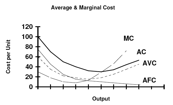
Average variable cost (AVC) represents the variable cost per unit of output, calculated as total variable cost divided by the quantity produced, and it specifically excludes fixed costs that do not fluctuate with production levels.^[4] This distinction is crucial in short-run economic analysis, where variable costs include expenses like labor and materials that vary directly with output volume, while fixed costs—such as rent or machinery depreciation—remain constant regardless of production quantity.^[1] For instance, in a bakery operation, variable costs might encompass flour and wages for additional bakers, but AVC ignores invariant elements like oven rental fees.^[5] In contrast to average fixed cost (AFC), which is total fixed cost divided by quantity and declines as output increases due to spreading fixed expenses over more units, AVC often exhibits a U-shaped curve with respect to output, initially falling due to efficiencies in variable input utilization before rising because of diminishing marginal returns to those inputs.^[6] AFC, being inversely related to output, approaches zero at high production levels, whereas AVC reflects the per-unit burden of scalable resources and often exhibits a U-shaped curve, initially falling due to efficiencies before rising from inefficiencies.^[4] This separation allows firms to isolate the impact of output changes on flexible costs alone. Average total cost (ATC), defined as total cost per unit or the sum of AVC and AFC, incorporates both variable and fixed components, providing a broader measure of overall production efficiency.^[1] Unlike AVC, which focuses solely on variable elements and thus lies below ATC on cost curves, ATC declines more gradually at low outputs due to falling AFC but eventually mirrors AVC's shape as fixed costs become negligible.^[6] For example, if a firm's AVC is $5 per unit at 100 units of output, but AFC adds $1, then ATC equals $6, highlighting how AVC understates total per-unit expenses.^[5] Marginal cost (MC), the additional cost of producing one more unit (change in total cost divided by change in quantity), differs from AVC as it measures incremental changes rather than averages, often intersecting AVC at its minimum point.^[1] In the short run, MC equals the change in variable cost per unit since fixed costs do not affect increments, but while AVC averages past variable costs, MC signals future cost trends and drives decisions on output expansion.^[6] This relationship underscores that when MC exceeds AVC, the average rises, but below it, AVC falls, aiding in optimizing production levels.^[4]

Mathematical Formulation

Formula Derivation

The average variable cost (AVC) is derived from the foundational concepts of total variable cost (TVC) and output quantity in the short run, where certain inputs like capital are fixed while others, such as labor, vary with production levels. TVC represents the sum of expenditures on variable inputs required to produce a given quantity of output

Q

. Assuming labor is the sole variable input with wage rate

w

, TVC is expressed as

\text{TVC}(Q) = w \cdot L(Q)

, where

L(Q)

is the quantity of labor needed to achieve output

Q

based on the production function.^[7] To obtain AVC, divide TVC by the output quantity:

\text{AVC}(Q) = \frac{\text{TVC}(Q)}{Q} = \frac{w \cdot L(Q)}{Q}.

This simplifies by recognizing that the average product of labor (APL) is

\text{APL}(Q) = \frac{Q}{L(Q)}

, the output per unit of labor. Rearranging yields:

\text{AVC}(Q) = w \cdot \frac{L(Q)}{Q} = \frac{w}{\text{APL}(Q)}.

Thus, AVC is the wage rate divided by the average product of the variable input, reflecting the inverse relationship between productivity and per-unit variable costs. This derivation assumes cost minimization, where the firm employs labor up to the point where the marginal product aligns with input prices, but the core formula holds for any short-run production scenario with variable labor costs. In more general cases with multiple variable inputs, TVC aggregates costs across all such inputs, and AVC remains

\frac{\text{TVC}(Q)}{Q}

, though the APL linkage applies primarily to single-input models.^[7]

Numerical Example

Consider a hypothetical bakery, Bob's Bakery, where fixed costs consist of a daily oven rental fee of $40, while variable costs include labor and ingredients that vary with the number of loaves produced. This example illustrates how average variable cost (AVC) is computed as total variable cost (TVC) divided by the quantity of output (Q).^[5] The following table presents data for two output levels, showing the relevant costs and the resulting AVC calculations:

Quantity (Q, loaves per day)	Total Variable Cost (TVC, $)	Average Variable Cost (AVC = TVC / Q, $ per loaf)
100	500	5.00
150	700	4.67

In this scenario, at 100 loaves, AVC is $500 / 100 = $5 per loaf. At 150 loaves, AVC decreases to $700 / 150 ≈ $4.67 per loaf, demonstrating the typical U-shaped pattern of the AVC curve in the short run due to initial economies of scale in variable inputs.^[5] This numerical illustration highlights AVC's role in assessing per-unit variable expenses, aiding firms in production decisions. For instance, the decline in AVC reflects spreading variable costs over more units, though it may eventually rise with diminishing returns.^[5]

Graphical Representation

Curve Characteristics

The average variable cost (AVC) curve is typically U-shaped, reflecting the per-unit variable costs of production as output increases in the short run. This shape arises because AVC, calculated as total variable cost divided by quantity produced (AVC = TVC / Q), initially declines as output rises, reaches a minimum point, and then increases thereafter. The curve's position lies entirely below the average total cost (ATC) curve, since ATC includes both variable and fixed costs (ATC = AVC + AFC), and the vertical distance between them equals the average fixed cost (AFC), which diminishes with higher output.^[8] The downward-sloping portion of the AVC curve occurs at low levels of output, where production benefits from increasing marginal returns to the variable input, such as labor. Here, each additional unit of input yields progressively larger increments in output, allowing variable costs to be spread over more units efficiently, thus reducing the average. For instance, in a manufacturing setting, initial hires might specialize tasks, boosting productivity and lowering per-unit variable expenses like wages and materials. This phase aligns with the early stages of the law of variable proportions, where efficiency gains dominate.^[9]^[10] At the minimum point of the AVC curve, the marginal cost (MC) curve intersects it from below, marking the output level where MC equals AVC. Beyond this point, the AVC curve slopes upward due to diminishing marginal returns, as further increases in the variable input lead to smaller output gains, raising the average variable cost per unit. This inflection reflects overcrowding of fixed factors, like plant capacity, causing inefficiencies such as higher material waste or overtime labor costs. The minimum AVC typically occurs at a lower output than the minimum ATC, since fixed costs continue to dilute even as variable costs rise.^[8]^[10] In graphical terms, the U-shape ensures the AVC curve serves as a short-run benchmark for firm decisions, with the MC curve crossing both AVC and ATC at their respective minima, pulling the averages downward when MC is below them and upward when above. This interaction underscores the curve's role in identifying efficient production scales before diseconomies set in.^[9]

Interaction with Marginal Cost

The interaction between average variable cost (AVC) and marginal cost (MC) is a fundamental principle in short-run production analysis, where MC influences the trajectory of the AVC curve. Marginal cost represents the additional cost of producing one more unit of output, calculated as the change in total variable cost divided by the change in output quantity (MC = ΔTVC / ΔQ). In contrast, AVC is the total variable cost per unit of output (AVC = TVC / Q). The key relationship arises because MC acts as the "driver" of AVC: when MC is below AVC, the AVC curve slopes downward, reflecting that the cost of additional units is pulling the average down; conversely, when MC exceeds AVC, the AVC curve slopes upward as higher marginal costs raise the average.^[11]^[12] This dynamic is most evident at the point where the MC curve intersects the AVC curve, which occurs precisely at the minimum of the AVC curve. At this intersection, MC equals AVC, marking the output level where average variable costs are lowest and production is at its most efficient in terms of variable inputs. Graphically, the typically U-shaped AVC curve is crossed by the MC curve from below at this minimum point, after which MC rises more steeply due to diminishing marginal returns. This intersection rule holds universally in standard microeconomic models, ensuring that firms can identify the optimal short-run output where variable costs per unit are minimized.^[13]^[11]^[12] The underlying mathematics reinforces this interaction: the derivative of total variable cost with respect to quantity yields MC, while AVC is the average of that function. As a result, the slope of AVC is positive when MC > AVC, zero when MC = AVC, and negative when MC < AVC, providing a rigorous basis for the curve behaviors observed in production functions. This principle, rooted in the broader relationship between marginal and average values in economics, aids firms in decision-making by highlighting how incremental costs affect overall efficiency.^[12]^[11]

Applications in Economics

Role in Short-Run Decisions

In the short run, where at least one input is fixed, firms must decide whether to produce output or temporarily shut down operations, and average variable cost (AVC) plays a central role in this analysis by representing the variable expenses per unit of output. Variable costs, such as labor and materials, can be avoided by halting production, whereas fixed costs like rent persist regardless. Thus, AVC determines whether revenue from sales can cover these avoidable costs, guiding loss-minimization strategies.^[14] The primary short-run decision rule involving AVC is the shutdown condition: a firm should cease production if the market price falls below the minimum point on its AVC curve, as continuing to operate would result in losses exceeding the fixed costs alone. At this point, total revenue would not cover total variable costs, making shutdown preferable to cover only fixed costs and avoid additional losses from variable inputs. For instance, in perfectly competitive markets, this rule ensures firms exit temporary low-price periods without depleting resources further. This shutdown point marks the lowest price at which the firm is willing to supply any output in the short run.^[15]^[16] When the price exceeds the minimum AVC, the firm opts to produce, selecting the output level where marginal cost equals marginal revenue to maximize profits or minimize losses, as this level allows coverage of all variable costs and a portion of fixed costs. The AVC curve thus defines the floor for the firm's short-run supply curve, which traces the marginal cost curve above the minimum AVC, reflecting how variable costs influence responsiveness to price changes. This framework applies across market structures, though it is most straightforward in competitive settings where firms are price takers.^[14]^[17]

Shutdown Analysis

In the short run, shutdown analysis for a perfectly competitive firm revolves around comparing the market price to the firm's average variable cost (AVC) to decide whether continued production minimizes losses. The core principle is that variable costs, such as labor and materials, can be avoided by halting output, while fixed costs like rent remain unavoidable regardless of production levels. If the price per unit falls below the minimum AVC, the firm incurs larger losses by operating than by shutting down, as total revenue fails to cover even the variable expenses. This decision framework ensures the firm selects the option that results in the smallest overall loss.^[18] The shutdown point occurs precisely at the minimum point on the AVC curve, where the marginal cost (MC) curve intersects it. At this intersection, the firm is indifferent between producing and shutting down, as price equals AVC, covering variable costs exactly but contributing nothing toward fixed costs. Below this point—when P < min AVC—revenue cannot offset variable outlays, so shutting down limits losses to the sunk fixed costs alone. For instance, a hypothetical raspberry farm with a minimum AVC of $1.65 per bushel would shut down if the market price drops to $1.50, resulting in total losses of $75, compared to losses equal to the fixed costs of $62 if shutting down. Conversely, if price equals or exceeds the minimum AVC (e.g., $1.70), the firm produces at the output where MC = P, covering variables and partially offsetting fixed costs to reduce net losses.^[18]^[19] Graphically, the shutdown region is depicted below the AVC curve on a cost-output diagram, with the MC curve rising through the U-shaped AVC. Firms operate along the MC curve above the AVC minimum during loss-making periods but exit production entirely in the shaded shutdown zone. This analysis underscores AVC's pivotal role in short-run viability, distinguishing temporary shutdowns from long-run exit decisions, where persistent losses below average total cost drive permanent closure. Empirical applications, such as in agricultural markets, highlight how volatile prices trigger shutdowns to preserve capital for potential recovery.^[18]^[20]

Info Pages

Talk Pages

Special Pages

Average variable cost

Recent from talks

Recent from talks

Contribute something

Contribute something

Media Pages

Timelines

Articles

Notes collections

Notes

Notes

Days in Chronicle

Average variable cost

See also

References