Configuration entropy Encyclopedia: Wikipedia & Grokipedia

Configuration entropy

current hub

Read side by side

Configuration entropy

View on Wikipedia

from Wikipedia

In statistical mechanics, configuration entropy is the portion of a system's entropy that is related to discrete representative positions of its constituent particles. For example, it may refer to the number of ways that atoms or molecules pack together in a mixture, alloy or glass, the number of conformations of a molecule, or the number of spin configurations in a magnet. The name might suggest that it relates to all possible configurations or particle positions of a system, excluding the entropy of their velocity or momentum, but that usage rarely occurs.^[1]

Calculation

[edit]

If the configurations all have the same weighting, or energy, the configurational entropy is given by Boltzmann's entropy formula

S=k_{B}\,\ln W,

where k_B is the Boltzmann constant and W is the number of possible configurations. In a more general formulation, if a system can be in states n with probabilities P_n, the configurational entropy of the system is given by

S=-k_{B}\,\sum _{n=1}^{W}P_{n}\ln P_{n},

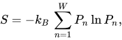
which in the perfect disorder limit (all P_n = 1/W) leads to Boltzmann's formula, while in the opposite limit (one configuration with probability 1), the entropy vanishes. This formulation is called the Gibbs entropy formula and is analogous to that of Shannon's information entropy.

The mathematical field of combinatorics, and in particular the mathematics of combinations and permutations is highly important in the calculation of configurational entropy. In particular, this field of mathematics offers formalized approaches for calculating the number of ways of choosing or arranging discrete objects; in this case, atoms or molecules. However, it is important to note that the positions of molecules are not strictly speaking discrete above the quantum level. Thus a variety of approximations may be used in discretizing a system to allow for a purely combinatorial approach. Alternatively, integral methods may be used in some cases to work directly with continuous position functions, usually denoted as a configurational integral.

Notes

[edit]

^ Hnizdo V, Gilson MK (March 2010). "Thermodynamic and Differential Entropy under a Change of Variables". Entropy. 12 (3): 578–590. Bibcode:2010Entrp..12..578H. doi:10.3390/e12030578. PMC 3891802. PMID 24436633.

References

[edit]

Kroemer H, Kittel C (1980). Thermal Physics (2nd ed.). W. H. Freeman Company. ISBN 978-0-7167-1088-2.

This article about statistical mechanics is a stub. You can help Wikipedia by expanding it.

This thermodynamics-related article is a stub. You can help Wikipedia by expanding it.

Revisions and contributors Edit on Wikipedia Read on Wikipedia

Configuration entropy

View on Grokipedia

from Grokipedia

Configurational entropy, often referred to as configuration entropy, quantifies the contribution to the total entropy of a system arising from the multiplicity of possible spatial or orientational arrangements of its constituent particles or molecules, distinct from contributions due to their velocities or internal vibrations. In statistical mechanics, it is formally expressed as $ S_{\text{conf}} = k_B \ln \Omega $, where $ k_B $ is Boltzmann's constant and $ \Omega $ represents the number of accessible microstates corresponding to those configurations at a given energy, volume, and particle number. This measure captures the inherent disorder associated with positional degrees of freedom, assuming the configurations are distinguishable and equally probable under equilibrium conditions.^[1]^[2] The total entropy of a system in statistical mechanics combines configurational entropy with thermal (or kinetic) entropy, which accounts for the distribution of momenta among particles; for classical systems, these are often separated via the phase space integral, with the configurational part derived from the spatial volume $ \int d\mathbf{r}_1 \cdots d\mathbf{r}N $ in the partition function. Changes in configurational entropy, $ \Delta S{\text{conf}} = k_B \ln (\Omega_2 / \Omega_1) $, drive processes where systems evolve toward states of higher multiplicity, such as mixing of ideal gases or conformational changes in molecules, provided energy dispersal is possible. In the Sackur-Tetrode equation for an ideal monatomic gas, the configurational component emerges from the $ V^N / N! $ term, reflecting positional randomness adjusted for particle indistinguishability.^[1]^[2] Configurational entropy plays a pivotal role across disciplines, influencing thermodynamic stability and phase behavior. In materials science and solid-state physics, it stabilizes disordered phases like alloys or glasses by contributing to the free energy minimization, calculated via methods such as cluster expansions or Monte Carlo sampling of the density of states; for instance, in binary alloys, it favors random site occupations at high temperatures. Notably, in recent years as of 2025, configurational entropy has been pivotal in the design of high-entropy alloys and materials, stabilizing multi-principal element compositions for advanced applications.^[3]^[4] In polymer and solution chemistry, it underlies the entropy of mixing in Flory-Huggins theory, where $ \Delta S_{\text{mix}} = -k_B (N_1 \ln \phi_1 + N_2 \ln \phi_2) $ promotes phase separation or solubility based on volume fractions. In biophysics, it governs noncovalent interactions, such as protein-ligand binding, where losses in rotational and translational freedom are offset by gains in internal conformational flexibility, often quantified using mutual information expansions from molecular dynamics simulations. These applications highlight its essential role in predicting equilibrium properties and designing materials or drugs.^[5]

Fundamentals

Definition

Configuration entropy, often denoted $ S_{\conf} $, is a measure in statistical mechanics that quantifies the degree of disorder associated with the number of possible microscopic arrangements or configurations of a system's particles or components, independent of their kinetic energies or internal states. It arises from the positional, orientational, or combinatorial degeneracy in the system's phase space and is formally expressed as $ S_{\conf} = k_B \ln \Omega $, where $ k_B $ is Boltzmann's constant and $ \Omega $ represents the number of accessible microstates consistent with the macroscopic constraints of the system. This formulation captures the entropic contribution from the multiplicity of ways particles can be distributed in space, emphasizing structural variability over energetic considerations.^[2] In contrast to the total entropy $ S $, which includes additive contributions from thermal motion (vibrational or kinetic degrees of freedom) and other internal processes, configuration entropy specifically isolates the degeneracy due to spatial or configurational freedom, such that $ S = S_{\conf} + S_{\thermal} + \cdots $. For systems where energy levels are degenerate or interactions are negligible, $ S_{\conf} $ dominates the positional disorder, ignoring fluctuations in momentum or potential energy that would contribute to thermal entropy. This distinction allows for a focused analysis of how structural arrangements drive thermodynamic behavior in dilute or ideal systems.^[2] The concept of configuration entropy originated with Ludwig Boltzmann's work in the late 19th century, particularly his 1877 paper that linked entropy to probability and the second law of thermodynamics through the logarithm of microstate multiplicity. A illustrative example appears in the entropy of a monatomic ideal gas, where the configurational component relates to the volume $ V $ and particle number $ N $ via the term $ N k_B \ln (V/N) $ in the Sackur-Tetrode equation, highlighting how increased volume enhances the number of positional configurations and thus entropy.^[6]^[2]

Relation to Statistical Mechanics

In statistical mechanics, the entropy $ S $ of a system is fundamentally defined as $ S = -k_B \sum_i p_i \ln p_i $, where $ k_B $ is Boltzmann's constant and $ p_i $ are the probabilities of the system's microstates. This Gibbs-Shannon formulation captures the uncertainty or disorder associated with the distribution of probabilities over accessible states. Configuration entropy emerges as a special case when all microstates are equally likely, such that $ p_i = 1/\Omega $ for $ \Omega $ total configurations, yielding $ S_\text{conf} = k_B \ln \Omega $.^[7] This limit applies to systems where energy differences are negligible compared to thermal energy, emphasizing the role of positional or structural arrangements in contributing to overall entropy./04%3A_Entropy/4.04%3A_Entropy_and_Information) The connection to the partition function arises in the canonical ensemble, where the total partition function $ Z = \sum_i e^{-\beta E_i} $ (with $ \beta = 1/(k_B T) $) sums over states weighted by their Boltzmann factors. For systems with highly degenerate energy levels—such as ideal mixtures or lattice models where configurations share the same energy—the configurational contribution dominates, simplifying to $ Z_\text{conf} \approx \Omega $.^[7] This leads to the Helmholtz free energy $ F = -k_B T \ln Z $, which decomposes into an energetic term plus a configurational entropy contribution $ -T S_\text{conf} $, highlighting how multiplicity of states lowers the free energy at finite temperatures.^[7] In such cases, the entropy itself derives from the free energy via $ S = -\partial F / \partial T $, underscoring the probabilistic foundation of thermodynamic potentials.^[7] Configuration entropy plays a pivotal role in establishing equilibrium, particularly in isothermal processes where it favors spontaneous changes like mixing or expansion to maximize $ \Omega $. In the Gibbs free energy $ \Delta G = \Delta H - T \Delta S_\text{conf} $, the entropic term balances enthalpic contributions, driving systems toward states of higher configurational disorder when $ \Delta G < 0 $. This mechanism explains phenomena such as ideal gas expansion or solute dissolution without energy barriers. For pure configurational effects to dominate, the system must satisfy the ergodic hypothesis, ensuring that time averages over trajectories equal ensemble averages over states, and remain isolated from external fields (e.g., gravitational or electromagnetic) that could bias configurations.^[8] These assumptions underpin the validity of treating configuration entropy as a standalone driver in equilibrium statistical mechanics.^[9]

Calculation Methods

Combinatorial Derivation

The combinatorial derivation of configurational entropy begins with the counting of microstates for a system of

N

indistinguishable particles confined to a volume

V

in classical statistical mechanics. Treating the positions as continuous requires discretizing the phase space into small cells to enable combinatorial counting; the number of accessible configurational microstates

\Omega

is then approximated as

\Omega \approx \frac{V^N}{N!}

, where the factorial accounts for the indistinguishability of the particles, ensuring that permutations among identical particles do not yield distinct states. This expression arises from initially considering distinguishable particles, which would give

\Omega = V^N

, and then dividing by

N!

to correct for overcounting due to indistinguishability.^[10] The configurational entropy

S_\text{conf}

follows from Boltzmann's relation

S = k_B \ln \Omega

, where

k_B

is Boltzmann's constant, yielding

S_\text{conf} = k_B \ln \left( \frac{V^N}{N!} \right) = k_B \left[ N \ln V - \ln N! \right]

. To evaluate this for large

N

, Stirling's approximation is applied:

\ln N! \approx N \ln N - N

. This simplifies the expression to

S_\text{conf} = k_B \left[ N \ln \left( \frac{V}{N} \right) + N \right],

which captures the entropy's dependence on the available volume per particle and the system's size.^[10] Stirling's approximation,

\ln N! \approx N \ln N - N + \frac{1}{2} \ln (2 \pi N)

, is valid for large

N

because it derives from the integral representation of the factorial via the gamma function or from asymptotic expansions of the sum

\ln N! = \sum_{k=1}^N \ln k

, which approximates the integral

\int_1^N \ln x \, dx = N \ln N - N + 1

. The leading term provides the dominant contribution in the thermodynamic limit

N \to \infty

, while higher-order terms like

\frac{1}{2} \ln (2 \pi N)

become negligible relative to

N

. For systems with distinguishable components, such as mixtures occupying

N

lattice sites with

n_A

particles of type A,

n_B

of type B, and so on where

\sum_i n_i = N

, the number of microstates is given by the multinomial coefficient

\Omega = \frac{N!}{n_A! n_B! \cdots}

, reflecting the ways to arrange the species while treating particles within each type as indistinguishable. The configurational entropy then becomes

S_\text{conf} = k_B \ln \Omega = -k_B \sum_i n_i \ln \left( \frac{n_i}{N} \right)

after applying Stirling's approximation to each factorial, which yields the standard entropy of mixing form.^[11] This expression highlights the contribution from compositional disorder and reduces to zero for pure systems where one

n_i = N

. The accuracy of these approximations depends on system size; for finite

N

, Stirling's formula incurs a relative error of order

O(1/N)

N!

, or

O(\ln N / N)

\ln N!

, which propagates to a small total correction in

S_\text{conf}

of roughly

-\frac{1}{2} k_B \ln (2 \pi N)

. In typical macroscopic systems with

N \sim 10^{23}

, this error is negligible, on the order of

10^{-22}

relative to the total entropy, justifying its use in the thermodynamic limit; however, for nanoscale or finite systems, exact factorial evaluations or refined Stirling series may be needed to avoid deviations up to a few percent.

Lattice Model Approaches

Lattice model approaches represent constrained environments, such as solids or polymer solutions, by discretizing space into a regular grid of sites, where each site is occupied by a component like A or B in binary systems. The configurational entropy arises from the number of ways Ω to arrange these components on the lattice, often computed using multinomial coefficients that distribute N_A particles of type A and N_B of type B across N total sites, while incorporating constraints such as nearest-neighbor exclusions to prevent unphysical overlaps or enforce bonding rules. This formulation captures spatial correlations absent in unconstrained models, providing a foundation for understanding mixing in ordered structures.^[12] In polymer applications, the Flory approximation simplifies the calculation of chain conformations by treating the polymer as a self-avoiding random walk on the lattice, estimating the number of valid configurations as approximately proportional to (z-1)^{N-1}, where z is the lattice coordination number and N is the chain length. The resulting configurational entropy is then S_{\text{conf}} \approx k_B \ln (\text{number of chain conformations}), which approximates the entropy loss upon placing multiple chains on the lattice while neglecting long-range excluded volume effects for tractability. This approach, central to early theories of polymer solutions, enables analytical estimates for dilute to semi-dilute regimes. Mean-field treatments average over all possible lattice configurations to derive an effective entropy expression, yielding S_{\text{conf}} = -k_B N [\phi \ln \phi + (1-\phi) \ln (1-\phi)], where \phi is the volume fraction of one component and N is the total number of sites; this assumes random mixing but can be refined with quasi-chemical corrections to account for short-range order induced by nearest-neighbor interactions. Developed independently by Flory and Huggins, this entropy term quantifies the ideal mixing contribution in binary lattice fluids and polymer blends, forming the basis for phase behavior predictions. Guggenheim's quasi-chemical approximation further enhances accuracy by modeling pair distributions as equilibrium "bonds," adjusting the entropy for non-random nearest-neighbor pairings without full enumeration. For large lattices where exact enumeration of Ω becomes computationally prohibitive, Monte Carlo sampling methods are employed to estimate the configurational entropy by generating statistically representative ensembles of arrangements and computing averages via thermodynamic integration or histogram reweighting techniques. These simulations handle complex constraints like exclusions efficiently, providing numerical benchmarks for mean-field predictions in systems with thousands of sites.^[13]

Applications in Physical Systems

Binary Mixtures

In binary mixtures, the configurational entropy of ideal mixing quantifies the increased disorder from randomly arranging two distinct molecular species. For a system with

N

total particles, the change in configurational entropy upon mixing is given by

\Delta S_{\text{mix}}^{\text{conf}} = -k_B N [x_A \ln x_A + x_B \ln x_B],

where

k_B

is Boltzmann's constant and

x_A

x_B

are the mole fractions of components A and B with

x_A + x_B = 1

. This formula derives from the Boltzmann relation

S = k_B \ln W

, where

W = N! / (N_A! N_B!)

represents the number of distinct arrangements assuming indistinguishable particles within each species and no volume change on mixing. The negative sign before the logarithmic terms ensures

\Delta S_{\text{mix}}^{\text{conf}} > 0

for

0 < x_i < 1

, as

\ln x_i < 0

, thereby providing a thermodynamic driving force for mixing even when enthalpic interactions are neutral or repulsive.^[14] This entropic contribution plays a central role in the thermodynamics of phase separation in binary mixtures, as described by regular solution theory. The molar Gibbs free energy of mixing is

\Delta G_{\text{mix}} = RT [x_A \ln x_A + x_B \ln x_B] + \Omega x_A x_B

, where

\Omega

is the interaction parameter reflecting enthalpic non-idealities. Stability analysis shows that the binodal curve, marking the boundary of phase separation, is influenced by the curvature of the entropic term; phase separation occurs for

\Omega > 2RT

, with the spinodal region defined where

\partial^2 \Delta G_{\text{mix}} / \partial x^2 < 0

. In symmetric cases where

\Omega

is composition-independent, the critical point occurs at

x_A = x_B = 0.5

, beyond which the entropic stabilization diminishes, promoting demixing at lower temperatures.^[15] Experimentally, configurational entropy dominates the behavior of binary mixtures in vapor-liquid equilibria at elevated temperatures, where kinetic energy minimizes enthalpic barriers and approaches ideal solution limits. For instance, in hydrocarbon-alcohol systems, high-temperature VLE data reveal near-ideal phase envelopes, with deviations from Raoult's law decreasing as the entropic term $ -R [x_A \ln x_A + x_B \ln x_B] $ outweighs interaction energies, facilitating complete vaporization and mixing. This is evident in distillation processes where thermal inputs enhance miscibility, underscoring the configurational entropy's role in predicting equilibrium compositions.^[16]^[17] A representative case is the ethanol-water binary mixture, commonly found in rubbing alcohol formulations, where configurational entropy drives miscibility despite partial enthalpic penalties from differing hydrogen-bonding strengths. The system exhibits complete solubility across all compositions at ambient and higher temperatures, with the ideal mixing entropy compensating for a negative excess entropy of approximately -5 to -10 J/mol·K in dilute regimes, resulting in an overall favorable

\Delta G_{\text{mix}}

. This entropy-driven behavior enables applications in solvent blending and extraction processes, highlighting practical implications in chemical engineering.^[18]

Polymer Solutions

In polymer solutions, the configurational entropy of mixing is described by the Flory-Huggins theory, which accounts for the disparity in molecular sizes between solvent molecules and long polymer chains. The theory posits that the entropy change upon mixing is given by

\Delta S_\text{conf} = -k_B \left[ n_s \ln \phi_s + n_p \ln \phi_p \right],

where

n_s

and

n_p

are the numbers of solvent molecules and polymer chains, respectively,

\phi_s

and

\phi_p

are their volume fractions, and corrections for chain length arise because the entropy contribution from polymers is scaled by the number of chains rather than the total number of monomers, reflecting the reduced translational freedom of entire macromolecules. This formulation, derived from a lattice model assuming random placement of chain segments, highlights how longer chains diminish the entropic gain from mixing compared to simple binary mixtures of small molecules.^[19] Beyond mixing entropy, the conformational entropy of individual polymer chains plays a crucial role in solution behavior, governing the chain's flexibility and spatial extension. For a single ideal chain with

N

monomers on a lattice, the conformational entropy is approximated as

S_\text{conf} \approx k_B \ln (z^N) = N k_B \ln z

, where

z

is the coordination number representing local bonding choices per monomer; this entropy decreases in dilute solutions due to solvation constraints that limit accessible conformations compared to the melt state. In concentrated solutions, interchain interactions further modulate this entropy, but the dominant effect remains the intrinsic randomness of chain folding. Theta solvents represent a special case where polymer-solvent interactions balance monomer-monomer repulsions, effectively setting the excluded volume parameter to zero and allowing chains to adopt ideal Gaussian conformations dominated by conformational entropy alone. In such conditions, the entropy gain from chain expansion precisely counters any residual volume exclusions, maintaining random coil statistics; deviations below the theta temperature favor attractions, triggering a coil-globule transition where the chain collapses into a compact state, incurring a significant loss of conformational entropy as the number of accessible configurations plummets. This transition underscores the delicate entropy-driven equilibrium in polymer solutions.^[20] A representative example is polyethylene-poly(ethylenepropylene) (PE-PEP) diblock copolymers dissolved in decane, where at elevated temperatures the PE blocks form extended coils, but cooling induces aggregation into crystalline cores surrounded by amorphous coronas, leading to entropy loss as the polymer segments sacrifice conformational freedom for ordered packing within lamellae of 40-80 Å thickness. This aggregation, driven by crystallization of the polyethylene blocks, reduces the overall configurational entropy of the system, stabilizing the macroaggregates observed via small-angle neutron scattering.^[21]

Extensions and Limitations

Non-Ideal Systems

In non-ideal systems, configurational entropy deviates from the ideal mixing approximation due to intermolecular correlations that restrict accessible microstates. In dense liquids, pair correlations reduce

S_\text{conf}

compared to the ideal gas value, with the excess configurational entropy

S^{ex}

quantified by integrating the radial distribution function

g(r)

over the pair correlation contribution:

S^{ex}_\text{pair}/Nk_B \approx -2\pi\rho \int_0^\infty [g(r)\ln g(r) - g(r) + 1] r^2 dr

, where

\rho

is the number density. This integral captures the loss of entropy from structural ordering, as demonstrated in simulations of Lennard-Jones fluids.^[22]^[23] Vibrational contributions complicate the isolation of true configurational entropy in solids, where low-frequency modes can mimic positional disorder but arise from lattice vibrations rather than atomic rearrangements. Distinguishing these requires separating the total entropy into vibrational (from phonon spectra) and configurational components, often via quasi-harmonic approximations that subtract harmonic vibrational entropy from the total to yield the anharmonic or defect-related

S_\text{conf}

. In alloys like

\alpha

-brass, this separation reveals that vibrational entropy changes with composition, but configurational entropy dominates mixing thermodynamics when vibrations are properly accounted for.^[24]^[25] In quantum systems, statistics for fermions and bosons further modify the number of accessible configurations

\Omega

beyond classical ideals. The Pauli exclusion principle enforces single occupancy per quantum state for fermions, eliminating configurations with multiple particles in the same state and yielding

S_\text{conf} = 0

for an ideal Fermi gas at

T=0

, as the ground state fills the lowest-energy states uniquely with no thermal or positional disorder. For bosons, Bose-Einstein condensation at low temperatures similarly collapses

\Omega

to the ground state, setting

S_\text{conf} \approx 0

, though without the exclusion constraint. Molecular dynamics simulations address these non-idealities by computing

S_\text{conf}

through histogram reweighting techniques, which reconstruct the density of states or probability distributions from biased ensembles. In this method, configurations from MD trajectories are reweighted using multiple histograms to estimate the partition function

Z

, enabling

S_\text{conf} = k_B \ln \Omega

via

Z = \int e^{-\beta U} d\mathbf{r}^N

, particularly useful for capturing correlations in liquids and solids. This approach has been applied to glass-forming liquids, achieving convergence for complex potentials where direct summation fails.^[26]^[27]

Experimental Measurement Challenges

Measuring the configurational entropy experimentally presents significant challenges, primarily due to the difficulty in isolating it from other entropy contributions within the total entropy of a system. Total entropy changes are typically determined through calorimetric techniques, such as differential scanning calorimetry (DSC), where the entropy increment is calculated as

\Delta S = \int \frac{C_p}{T} \, dT

, with

C_p

being the heat capacity at constant pressure and

T

the temperature.^[28] However, this total entropy includes vibrational, rotational, translational, and electronic components, necessitating their subtraction to isolate the configurational part, which arises from the multiplicity of atomic or molecular arrangements.^[29] Deconvoluting these contributions often relies on spectroscopic methods to quantify the non-configurational terms. Vibrational entropy, for instance, can be estimated from inelastic neutron scattering or Raman/infrared spectroscopy by analyzing phonon densities of states, allowing subtraction from the calorimetric total to yield

S_\text{conf}

.^[29] Electronic entropy may be approximated using magnetic susceptibility measurements or electronic structure calculations, though these introduce additional approximations. In practice, such separations are imprecise for complex systems, as assumptions about mode independence or ideal behavior can lead to errors exceeding 10-20% in

S_\text{conf}

estimates.^[28] Specific techniques have been developed to probe configurational aspects indirectly. In polymer systems, neutron scattering, particularly small-angle neutron scattering (SANS), reveals chain conformations and segmental dynamics, from which configurational entropy related to polymer flexibility can be inferred through models of Gaussian chains or reptation.^[30] For binary mixtures or alloys, small-angle X-ray scattering (SAXS) provides information on density fluctuations and phase separation, enabling estimation of the degeneracy

\Omega

via scattering structure factors that reflect configurational disorder.^[31] These methods, while powerful, require complementary simulations to translate structural data into entropy values and are limited to accessible length scales (1-100 nm). Uncertainties in these measurements often stem from assumptions of ideality, where deviations due to interactions are neglected, leading to overestimation or underestimation of

S_\text{conf}

. In protein folding, for example, configurational entropy is estimated from unfolding free energies

\Delta G_\text{unfold}

, assuming

\Delta S_\text{conf} \approx -T^{-1} (\Delta G_\text{unfold} - \Delta H_\text{unfold})

, yielding losses of approximately 5-15

k_B

per residue; however, correlations between residues and solvent effects introduce uncertainties up to 30% in these values.^[32]^[33] Historically, early 20th-century efforts to measure mixing entropy in alloys faced substantial hurdles, as calorimeters like the Kawakami design in the 1920s struggled with precise heat-of-mixing determinations amid phase segregation and non-ideal behaviors, sparking debates on whether observed entropies matched ideal solution predictions.^[34] These issues were largely resolved by mid-century advances in high-temperature calorimetry and solution thermodynamics, enabling more accurate verification of configurational contributions in metallic systems.^[35]

Knowledge Base

Talk Channels

Special Pages

Configuration entropy

Configuration entropy

Configuration entropy

Calculation

See also

Notes

References

Configuration entropy

Fundamentals

Definition

Relation to Statistical Mechanics

Calculation Methods

Combinatorial Derivation

Lattice Model Approaches

Applications in Physical Systems

Binary Mixtures

Polymer Solutions

Extensions and Limitations

Non-Ideal Systems

Experimental Measurement Challenges

References

History

Configuration entropy

Configuration entropy

Configuration entropy

Calculation

See also

Notes

References

Configuration entropy

Fundamentals

Definition

Relation to Statistical Mechanics

Calculation Methods

Combinatorial Derivation

Lattice Model Approaches

Applications in Physical Systems

Binary Mixtures

Polymer Solutions

Extensions and Limitations

Non-Ideal Systems

Experimental Measurement Challenges

References