Hubbry Logo
Non-random two-liquid modelNon-random two-liquid modelMain
Open search
Non-random two-liquid model
Community hub
Non-random two-liquid model
logo
8 pages, 0 posts
0 subscribers
Be the first to start a discussion here.
Non-random two-liquid model
from Wikipedia
VLE of the mixture of chloroform and methanol plus NRTL fit and extrapolation to different pressures

The non-random two-liquid model[1] (abbreviated NRTL model) is an activity coefficient model introduced by Renon and Prausnitz in 1968 that correlates the activity coefficients of a compound with its mole fractions in the liquid phase concerned. It is frequently applied in the field of chemical engineering to calculate phase equilibria. The concept of NRTL is based on the hypothesis of Wilson, who stated that the local concentration around a molecule in most mixtures is different from the bulk concentration. This difference is due to a difference between the interaction energy of the central molecule with the molecules of its own kind and that with the molecules of the other kind . The energy difference also introduces a non-randomness at the local molecular level. The NRTL model belongs to the so-called local-composition models. Other models of this type are the Wilson model, the UNIQUAC model, and the group contribution model UNIFAC. These local-composition models are not thermodynamically consistent for a one-fluid model for a real mixture due to the assumption that the local composition around molecule i is independent of the local composition around molecule j. This assumption is not true, as was shown by Flemr in 1976.[2][3] However, they are consistent if a hypothetical two-liquid model is used.[4] Models, which have consistency between bulk and the local molecular concentrations around different types of molecules are COSMO-RS, and COSMOSPACE.

Derivation

[edit]

Like Wilson (1964), Renon & Prausnitz (1968) began with local composition theory,[5] but instead of using the Flory–Huggins volumetric expression as Wilson did, they assumed local compositions followed

with a new "non-randomness" parameter α. The excess Gibbs free energy was then determined to be

.

Unlike Wilson's equation, this can predict partially miscible mixtures. However, the cross term, like Wohl's expansion, is more suitable for than , and experimental data is not always sufficiently plentiful to yield three meaningful values, so later attempts to extend Wilson's equation to partial miscibility (or to extend Guggenheim's quasichemical theory for nonrandom mixtures to Wilson's different-sized molecules) eventually yielded variants like UNIQUAC.

Equations for a binary mixture

[edit]

For a binary mixture the following functions[6] are used:

with

Here, and are the dimensionless interaction parameters, which are related to the interaction energy parameters and by:

Here R is the gas constant and T the absolute temperature, and Uij is the energy between molecular surface i and j. Uii is the energy of evaporation. Here Uij has to be equal to Uji, but is not necessary equal to .

The parameters and are the so-called non-randomness parameter, for which usually is set equal to . For a liquid, in which the local distribution is random around the center molecule, the parameter . In that case, the equations reduce to the one-parameter Margules activity model:

In practice, is set to 0.2, 0.3 or 0.48. The latter value is frequently used for aqueous systems. The high value reflects the ordered structure caused by hydrogen bonds. However, in the description of liquid-liquid equilibria, the non-randomness parameter is set to 0.2 to avoid wrong liquid-liquid description. In some cases, a better phase equilibria description is obtained by setting .[7] However this mathematical solution is impossible from a physical point of view since no system can be more random than random (). In general, NRTL offers more flexibility in the description of phase equilibria than other activity models due to the extra non-randomness parameters. However, in practice this flexibility is reduced in order to avoid wrong equilibrium description outside the range of regressed data.

The limiting activity coefficients, also known as the activity coefficients at infinite dilution, are calculated by:

The expressions show that at , the limiting activity coefficients are equal. This situation occurs for molecules of equal size but of different polarities.
It also shows, since three parameters are available, that multiple sets of solutions are possible.

General equations

[edit]

The general equation for for species in a mixture of components is:[8]

with

There are several different equation forms for and , the most general of which are shown above.

Temperature dependent parameters

[edit]

To describe phase equilibria over a large temperature regime, i.e. larger than 50 K, the interaction parameter has to be made temperature dependent. Two formats are frequently used. The extended Antoine equation format:

Here the logarithmic and linear terms are mainly used in the description of liquid-liquid equilibria (miscibility gap).

The other format is a second-order polynomial format:

Parameter determination
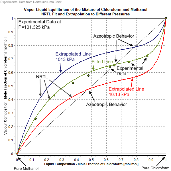
[edit]

The NRTL parameters are fitted to activity coefficients that have been derived from experimentally determined phase equilibrium data (vapor–liquid, liquid–liquid, solid–liquid) as well as from heats of mixing. The source of the experimental data are often factual data banks like the Dortmund Data Bank. Other options are direct experimental work and predicted activity coefficients with UNIFAC and similar models. It is noteworthy that for the same mixture several NRTL parameter sets might exist, and the choice of NRTL parameter set depends on the kind of phase equilibrium (i.e. solid–liquid (SL), liquid–liquid (LL), vapor–liquid (VL)). In the case of vapor–liquid equilibria, the fitted result importantly depends on which saturated vapor pressure of the pure components was used, and whether the gas phase was treated as an ideal or a real gas. Accurate saturated vapor pressure values are important in the determination or the description of an azeotrope. The gas fugacity coefficients are mostly set to unity (ideal gas assumption), but for vapor-liquid equilibria at high pressures (i.e. > 10 bar) an equation of state is needed to calculate the gas fugacity coefficient for a real gas description.

Determination of NRTL parameters from regression of LLE and VLE experimental data is a challenging problem because it involves solving isoactivity or isofugacity equations which are highly non-linear. In addition, parameters obtained from LLE of VLE may not always represent the experimental behaviour expected.[9][10][11] For this reason it is necessary to confirm the thermodynamic consistency of the obtained parameters in the whole range of compositions (including binary subsystems, experimental and calculated tie-lines, calculated plait point locations from the Hessian matrix, etc.) by using a phase stability test such as the Gibbs free energy minor tangent criteria.[12][13][14]

Parameters for NRTL model

[edit]

NRTL binary interaction parameters have been published in the Dechema data series and are provided by NIST and DDBST. There also exist machine-learning approaches that are able to predict NRTL parameters by using the SMILES notation for molecules as input.[15]

Literature

[edit]
  1. ^ Renon, Henri; Prausnitz, J. M. (January 1968). "Local compositions in thermodynamic excess functions for liquid mixtures". AIChE Journal. 14 (1): 135–144. Bibcode:1968AIChE..14..135R. doi:10.1002/aic.690140124.
  2. ^ McDermott, C.; Ashton, N. (January 1977). "Note on the definition of local composition". Fluid Phase Equilibria. 1 (1): 33–35. doi:10.1016/0378-3812(77)80024-1.
  3. ^ Flemr, V. (1976). "A note on excess Gibbs energy equations based on local composition concept". Collection of Czechoslovak Chemical Communications. 41 (11): 3347–3349. doi:10.1135/cccc19763347.
  4. ^ Hu, Y.; Azevedo, E.G.; Prausnitz, J.M. (January 1983). "The molecular basis for local compositions in liquid mixture models". Fluid Phase Equilibria. 13: 351–360. doi:10.1016/0378-3812(83)80106-X.
  5. ^ Renon, Henri; Prausnitz, J. M. (January 1968). "Local compositions in thermodynamic excess functions for liquid mixtures". AIChE Journal. 14 (1): 135–144. Bibcode:1968AIChE..14..135R. doi:10.1002/aic.690140124.
  6. ^ Reid, Robert C.; Prausnitz, J. M.; Poling, Bruce E. (1987). The Properties of Gases and Liquids. McGraw-Hill. ISBN 978-0-07-051799-8.[page needed]
  7. ^ Marina, J. M.; Tassios, D. P. (January 1973). "Effective Local Compositions in Phase Equilibrium Correlations". Industrial & Engineering Chemistry Process Design and Development. 12 (1): 67–71. doi:10.1021/i260045a013.
  8. ^ "A Property Methods and Calculations" (PDF). Rowan University.
  9. ^ Reyes-Labarta, J.A.; Olaya, M.M.; Velasco, R.; Serrano, M.D.; Marcilla, A. (April 2009). "Correlation of the liquid–liquid equilibrium data for specific ternary systems with one or two partially miscible binary subsystems". Fluid Phase Equilibria. 278 (1–2): 9–14. doi:10.1016/j.fluid.2008.12.002.
  10. ^ Marcilla Gomis, Antonio (4 November 2011). "GE Models and Algorithms for Condensed Phase Equilibrium Data Regression in Ternary Systems: Limitations and Proposals". The Open Thermodynamics Journal. 5 (1): 48–62. doi:10.2174/1874396X01105010048. hdl:10045/19865.
  11. ^ Marcilla, A.; Serrano, M.D.; Reyes-Labarta, J.A.; Olaya, M.M. (4 April 2012). "Checking Liquid–Liquid Plait Point Conditions and Their Application in Ternary Systems". Industrial & Engineering Chemistry Research. 51 (13): 5098–5102. doi:10.1021/ie202793r.
  12. ^ Li, Zheng; Smith, Kathryn H.; Mumford, Kathryn A.; Wang, Yong; Stevens, Geoffrey W. (July 2015). "Regression of NRTL parameters from ternary liquid–liquid equilibria using particle swarm optimization and discussions". Fluid Phase Equilibria. 398: 36–45. doi:10.1016/j.fluid.2015.04.006. hdl:10045/66521.
  13. ^ Labarta, Juan A.; Olaya, Maria del Mar; Marcilla, Antonio (27 November 2015). GMcal_TieLinesLL: Graphical User Interface (GUI) for the Topological Analysis of Calculated GM Surfaces and Curves, including Tie-Lines, Hessian Matrix, Spinodal Curve, Plait Point Location, etc. for Binary and Ternary Liquid -Liquid Equilibrium (LLE) Data (Report). hdl:10045/51725.
  14. ^ Labarta, Juan A.; Olaya, Maria del Mar; Marcilla, Antonio (7 April 2022). GMcal_TieLinesVL: Graphical User Interface (GUI) for the Topological Analysis of Experimental and Calculated GM Functions for Binary and Ternary (Isobaric or Isothermal) Vapor-Liquid Equilibrium (VLE or VLLE) Data (including Tie-Lines, Derivatives, Distillation Boundaries, LL Critical Points Location, etc.) (Report). hdl:10045/122857.
  15. ^ Winter, Benedikt; Winter, Clemens; Esper, Timm; Schilling, Johannes; Bardow, André (May 2023). "SPT-NRTL: A physics-guided machine learning model to predict thermodynamically consistent activity coefficients". Fluid Phase Equilibria. 568 113731. arXiv:2209.04135. doi:10.1016/j.fluid.2023.113731.
Revisions and contributorsEdit on WikipediaRead on Wikipedia
from Grokipedia
The non-random two-liquid (NRTL) model is a coefficient model designed to represent the non-ideal behavior of multicomponent mixtures, particularly for calculating phase equilibria such as vapor- (VLE) and - (LLE) equilibria. It assumes that the local composition around a central in the phase differs from the bulk composition due to differences in intermolecular interactions, leading to non-random molecular arrangements. Developed by Henri Renon and John M. Prausnitz in 1968, the NRTL model builds on the two-liquid theory proposed by R.L. Scott and the local composition concept introduced by Grant M. Wilson, extending these ideas to derive an expression for the excess Gibbs free energy of mixing. The model's core formulation expresses the molar excess Gibbs energy (GEG^E) as GERT=ixijxjGjiτjikxkGki\frac{G^E}{RT} = \sum_i x_i \frac{\sum_j x_j G_{ji} \tau_{ji}}{\sum_k x_k G_{ki}}, where xix_i is the mole fraction of component ii, Gji=exp(αjiτji)G_{ji} = \exp(-\alpha_{ji} \tau_{ji}), and τji=gjigiiRT\tau_{ji} = \frac{g_{ji} - g_{ii}}{RT}, with gjig_{ji} representing the energetic interaction between molecules jj and ii, RR the gas constant, and TT the temperature. Activity coefficients (γi\gamma_i) are then obtained by differentiating this expression, enabling predictions of phase behavior from binary interaction parameters. The NRTL model requires three adjustable parameters per binary pair: two binary interaction parameters (τij\tau_{ij} and τji\tau_{ji}, related to energy differences) and a non-randomness factor (αij\alpha_{ij}, typically fixed between 0.2 and 0.47 to reflect the degree of local order, though it can be adjustable). These parameters are regressed from experimental data, such as VLE or LLE measurements, making the model empirical yet versatile for systems exhibiting partial or azeotropes. Widely applied in for and design— including , extraction, and reactive systems—the NRTL model excels in handling both polar and non-polar mixtures but can face challenges with highly nonlinear behavior, parameter inconsistency across temperature ranges, and convergence issues in multicomponent calculations. Extensions like the electrolyte NRTL (eNRTL) have adapted it for ionic solutions, enhancing its utility in areas such as CO₂ capture and battery electrolytes.

Introduction

Overview

The non-random two-liquid (NRTL) model is an model designed to correlate mole fraction-based s (γi\gamma_i) in multicomponent nonelectrolyte mixtures, accurate representation of non-ideal solution . Developed by Renon and Prausnitz in 1968, it builds on local composition concepts to address limitations in prior models that assumed random molecular mixing, such as the Margules and van Laar equations. At its core, the NRTL model accounts for non-random local compositions around a central , which arise due to differing interaction energies between like pairs (UiiU_{ii}) and unlike pairs (UijU_{ij}) in the mixture. This approach recognizes that molecules tend to associate preferentially with similar species in non-ideal systems, leading to deviations from bulk composition. The model incorporates two binary energy τij\tau_{ij} and τji\tau_{ji} (reflecting interaction energy differences) and a non-randomness αij\alpha_{ij} (typically between 0.2 and 0.47, controlling the degree of local order), where the term Gij=exp(αijτij)G_{ij} = \exp(-\alpha_{ij} \tau_{ij}) accounts for non-randomness in local composition. In , the NRTL model is widely applied to predict phase equilibria, including vapor-liquid equilibria for processes, liquid-liquid equilibria for extraction operations, and solid-liquid equilibria for and calculations. These applications rely on the model's ability to fit experimental data with a minimal number of adjustable parameters, making it suitable for multicomponent systems without requiring additional terms beyond binary interactions.

Historical Development

The non-random two-liquid (NRTL) model was introduced in 1968 by Henri Renon and J. M. Prausnitz in their seminal paper published in the AIChE Journal. This work derived a new expression for the excess Gibbs energy of liquid mixtures based on local composition concepts, extending prior thermodynamic frameworks to better handle nonideal behaviors. The primary for developing the NRTL model stemmed from the limitations of the Wilson equation, introduced in 1964, which excelled at correlating vapor-liquid equilibria in fully systems but failed to predict phase splitting or partial miscibility in strongly nonideal liquids. Renon and Prausnitz addressed this by incorporating a nonrandomness factor into a two-liquid approximation, enabling the model to represent liquid-liquid equilibria and ternary systems using only binary parameters, thus providing greater versatility for complex mixtures. By the 1980s, the NRTL model had gained widespread adoption in chemical , with integration into commercial software such as Aspen Plus, facilitating its use in and optimization of separation processes. This early incorporation into tools accelerated its application in practice, where it remains a standard for calculations in nonideal systems. In recent years, advancements have focused on enhancing parameter estimation efficiency, exemplified by approaches that predict NRTL interaction parameters from molecular representations like SMILES strings. A notable 2023 study introduced the SPT-NRTL model, a physics-guided that ensures thermodynamic consistency while enabling rapid predictions for diverse mixtures, building on the original framework for modern computational workflows.

Theoretical Basis

Local Composition Concept

The local composition concept in the non-random two-liquid (NRTL) model describes how the composition of a varies at the molecular level, specifically around a central of one component. The local of component jj surrounding a central of component ii, denoted xjix_{ji}, deviates from the overall bulk xjx_j because molecules tend to associate preferentially with neighbors that minimize the system's energy, favoring unlike interactions over random distribution. This idea accounts for the non-ideal behavior in mixtures where intermolecular forces lead to clustering or segregation at short ranges. In contrast to random mixing assumptions, where local and bulk compositions are identical—as in solutions with no energetic biases—the NRTL model incorporates non-randomness driven by differences in pairwise interaction energies. Under random mixing, molecules distribute uniformly without preference, resulting in zero excess Gibbs energy beyond . The NRTL approach, however, posits that stronger attractive forces between unlike pairs (or weaker repulsive forces) cause deviations, making the local environment richer or poorer in certain components compared to the bulk. This non-random arrangement is assumed to be proportional to the relative differences, providing a more realistic depiction of real liquid mixtures exhibiting azeotropes or phase splitting. The NRTL model builds upon the local composition framework first proposed by Wilson in 1964, which introduced the idea that activity coefficients could be derived from local rather than bulk compositions to better capture non-idealities. While Wilson's model assumes a regular, random local structure adjusted only by interaction energies, NRTL extends this by adding a non-randomness parameter αij\alpha_{ij} (typically between 0.2 and 0.47) to explicitly measure the extent of deviation from randomness, allowing it to handle systems with significant local order, such as those forming two liquid phases. This enhancement makes NRTL particularly suitable for partially miscible systems. Intuitively, the local composition in NRTL is captured by the relation xji=xjexp(αjiτji)kxkexp(αkiτki)x_{ji} = \frac{x_j \exp(-\alpha_{ji} \tau_{ji})}{\sum_k x_k \exp(-\alpha_{ki} \tau_{ki})}, where τji=gjigiiRT\tau_{ji} = \frac{g_{ji} - g_{ii}}{RT} quantifies the energetic disparity between jj-ii and ii-ii interactions relative to thermal energy RTRT, with RR the and TT the temperature. The parameter τji\tau_{ji}, tied to binary interaction energies, is explored further in the model parameters section. This formulation ensures that local compositions sum to unity and reflect the model's two-liquid hypothesis of microphase separation.

Key Assumptions

The Non-random two-liquid (NRTL) model is grounded in the two-liquid hypothesis, which conceptualizes a as a superposition of two immiscible "pure" phases, each characterized by local enrichment in one component, thereby accounting for compositional heterogeneities at the molecular level. This approach, originally developed by Scott and adapted by Renon and Prausnitz, enables the model to describe both miscible and partially immiscible systems by treating the overall as a blend of these hypothetical liquids. A core assumption is that local compositions are derived from bulk compositions using a quasi-lattice approximation that posits molecules occupy lattice sites with surrounding coordination shells. This simplification allows for the definition of local mole fractions to capture non-ideal behavior without requiring detailed knowledge of the global arrangement, facilitating practical computations. The model further assumes that molecular interactions occur exclusively in pairwise fashion, focusing on binary energy parameters between unlike and disregarding higher-order multiplet effects to maintain tractability. and effects are incorporated primarily via the model's adjustable parameters, such as the dimensionless energy difference τij\tau_{ij}, which exhibits temperature dependence through forms like τij=aij+bijT\tau_{ij} = a_{ij} + \frac{b_{ij}}{T}, where aija_{ij} and bijb_{ij} are fitted constants, RR is the , and TT is . The NRTL framework is designed for systems with moderate to strong deviations from ideality, such as those prone to phase splitting, but presumes no dominant associative interactions (e.g., strong hydrogen bonding) that would require additional modifications for accurate representation. The degree of non-randomness in these local environments is quantified by the αij\alpha_{ij}, typically ranging from 0.2 (for hydrocarbons with polar liquids) to 0.47 (for self-associating systems).

Derivation of the Model

Excess Gibbs Energy Expression

The molar excess in the non-random two-liquid (NRTL) model is derived from principles of local compositions, assuming that the local composition around a central differs from the bulk due to non-random molecular arrangements from differences in intermolecular interactions. This extends earlier two-liquid theories by incorporating a non-randomness factor to account for preferential interactions in the coordination shells around each central . The full expression for the molar excess Gibbs free energy in a multicomponent mixture is given by GexRT=ixijτjiGjixjkGkixk,\frac{G^{ex}}{RT} = \sum_i x_i \frac{\sum_j \tau_{ji} G_{ji} x_j}{\sum_k G_{ki} x_k}, where xix_i is the global mole fraction of component ii, τji=gjigiiRT\tau_{ji} = \frac{g_{ji} - g_{ii}}{RT} represents the dimensionless energetic interaction parameter between molecules jj and ii relative to the pure ii component (with gjig_{ji} denoting the molar interaction energy of jj-ii pairs, and giig_{ii} for ii-ii pairs), and Gji=exp(αjiτji)G_{ji} = \exp(-\alpha_{ji} \tau_{ji}) is the nonrandomness factor incorporating the parameter αji\alpha_{ji} (typically 0.2–0.47, reflecting the degree of local order). This formulation arises from approximating the residual excess Gibbs energy using local mole fractions, where the first summation term in the equation captures deviations from random mixing due to preferential interactions. The NRTL expression relates to the classical two-liquid model by treating the mixture as a weighted superposition of local "liquid" environments around each component, with corrections for nonrandomness that adjust the effective compositions beyond simple volume averaging of pure component properties. This approach enables the model to predict liquid-liquid immiscibility and other phase behaviors by allowing GexG^{ex} to exhibit common tangent constructions. From this excess Gibbs energy, activity coefficients can be obtained via the Gibbs-Duhem relation, though detailed formulations appear elsewhere.

Activity Coefficient Formulation

The activity coefficient for component ii in the non-random two-liquid (NRTL) model is obtained by differentiating the molar excess Gibbs energy GE/RTG^E/RT with respect to the mole number of component ii, while holding temperature TT, pressure PP, and the mole numbers of other components constant: lnγi=((nGE/RT)ni)T,P,nj\ln \gamma_i = \left( \frac{\partial (n G^E / RT)}{\partial n_i} \right)_{T,P,n_j}. This partial derivative yields the explicit expression for lnγi\ln \gamma_i, which takes a two-term form reflecting the model's local composition and asymmetry corrections. The first term captures the local composition correction around component ii: jxjτjiGjikxkGki\frac{\sum_j x_j \tau_{ji} G_{ji}}{\sum_k x_k G_{ki}} where xjx_j is the liquid of component jj, τji=(gjigii)/RT\tau_{ji} = (g_{ji} - g_{ii})/RT with gjig_{ji} representing the energetic interaction between molecules jj and ii, and Gji=exp(αjiτji)G_{ji} = \exp(-\alpha_{ji} \tau_{ji}) incorporating the non-randomness αji\alpha_{ji}. This term adjusts the random mixing assumption by accounting for non-ideal local environments. The second term addresses the in local compositions for unlike pairs: jxjGijkxkGkj(τijmxmτmjGmjkxkGkj)\sum_j \frac{x_j G_{ij}}{\sum_k x_k G_{kj}} \left( \tau_{ij} - \frac{\sum_m x_m \tau_{mj} G_{mj}}{\sum_k x_k G_{kj}} \right) This correction ensures the model can represent systems where the local mole fractions differ between surrounding , arising from the unsymmetry in interaction energies (τijτji\tau_{ij} \neq \tau_{ji}). In limiting cases, the formulation satisfies thermodynamic expectations: as the xi1x_i \to 1, γi1\gamma_i \to 1, recovering ideal behavior in pure components; as xi0x_i \to 0, γi\gamma_i^\infty emerges from the infinite dilution interactions, quantified by the τ\tau and GG terms specific to the surrounding dominant component. The model's structure inherently promotes Gibbs-Duhem consistency at constant and , particularly in ideal or near-ideal limits, by deriving γi\gamma_i directly from the excess Gibbs energy expression.

Equations for Mixtures

Binary Mixtures

The Non-random two-liquid (NRTL) model simplifies for binary mixtures consisting of components 1 and 2, where the activity coefficients are expressed in terms of mole fractions x1x_1 and x2=1x1x_2 = 1 - x_1, binary interaction parameters τij\tau_{ij}, and nonrandomness factors GijG_{ij}. The natural logarithm of the for component 1 is given by lnγ1=x22[τ21G21(x1+x2G21)2+τ12G12(x2+x1G12)2],\ln \gamma_1 = x_2^2 \left[ \frac{\tau_{21} G_{21}}{(x_1 + x_2 G_{21})^2} + \frac{\tau_{12} G_{12}}{(x_2 + x_1 G_{12})^2} \right], and symmetrically for component 2, lnγ2=x12[τ12G12(x2+x1G12)2+τ21G21(x1+x2G21)2].\ln \gamma_2 = x_1^2 \left[ \frac{\tau_{12} G_{12}}{(x_2 + x_1 G_{12})^2} + \frac{\tau_{21} G_{21}}{(x_1 + x_2 G_{21})^2} \right]. Here, Gij=exp(αijτij)G_{ij} = \exp(-\alpha_{ij} \tau_{ij}), with τij=(gijgjj)/RT\tau_{ij} = (g_{ij} - g_{jj})/RT representing dimensionless energy differences between interaction parameters gijg_{ij}, the gas constant RR, and TT; αij\alpha_{ij} is the nonrandomness parameter, typically between 0.2 and 0.47 for binary systems. These forms arise from the local composition concept applied to two-liquid , enabling representation of nonideal behavior in binary liquid phases. At infinite dilution, the activity coefficients exhibit limiting behavior that highlights extreme nonidealities. For component 1 as x10x_1 \to 0, lnγ1=τ21exp(α21τ21)+τ12exp(α12τ12),\ln \gamma_1^\infty = \tau_{21} \exp(\alpha_{21} \tau_{21}) + \tau_{12} \exp(-\alpha_{12} \tau_{12}), and symmetrically for component 2 as x20x_2 \to 0, lnγ2=τ12exp(α12τ12)+τ21exp(α21τ21).\ln \gamma_2^\infty = \tau_{12} \exp(\alpha_{12} \tau_{12}) + \tau_{21} \exp(-\alpha_{21} \tau_{21}). These limits provide key insights into and partitioning, as they quantify the when one component is present in trace amounts. A representative example is the ethanol(1)-water(2) binary mixture at 25°C, where typical NRTL parameters are α12=0.3\alpha_{12} = 0.3, τ12=3.4578\tau_{12} = 3.4578, and τ21=0.8009\tau_{21} = -0.8009. These yield activity coefficient curves showing positive deviations from Raoult's law, with γ1\gamma_1 ranging from approximately 1.5 at equimolar composition to over 4 at low ethanol concentrations, and γ2\gamma_2 peaking near 6 at low water concentrations. The parameters align well with experimental vapor-liquid equilibrium data. The binary NRTL equations effectively capture both positive and negative deviations from ideality, as well as the formation of in systems like ethanol-water, which exhibits a minimum-boiling at about 89 mol% due to the asymmetric promoting phase splitting tendencies in the model framework.

Multicomponent Systems

The Non-random two-liquid (NRTL) model extends naturally to multicomponent mixtures with n>2n > 2 components through generalized summation forms that account for all pairwise interactions. The for component ii in an nn-component mixture is given by lnγi=jxjτjiGjikxkGki+jxjGijkxkGkj(τijmxmτmjGmjkxkGkj),\ln \gamma_i = \frac{\sum_j x_j \tau_{ji} G_{ji}}{\sum_k x_k G_{ki}} + \sum_j \frac{x_j G_{ij}}{\sum_k x_k G_{kj}} \left( \tau_{ij} - \frac{\sum_m x_m \tau_{mj} G_{mj}}{\sum_k x_k G_{kj}} \right), where xjx_j is the liquid mole fraction of component jj, τij\tau_{ij} is the non-randomness energy parameter between components ii and jj, and GijG_{ij} is the local composition Boltzmann factor defined for all pairs as Gij=exp(αijτij).G_{ij} = \exp(-\alpha_{ij} \tau_{ij}). Here, αij\alpha_{ij} represents the non-randomness parameter, typically between 0 and 1, which measures the degree of local order in the mixture. This formulation requires binary interaction parameters τij\tau_{ij} and αij\alpha_{ij} (or τji\tau_{ji}, αji\alpha_{ji}) for every unique pair of components, resulting in a parameter matrix that scales quadratically with the number of components. In practice, computing activity coefficients for vapor-liquid equilibrium (VLE) in multicomponent systems involves iterative numerical solutions because the vapor mole fractions yiy_i depend implicitly on the liquid compositions xix_i via yi=xiγiPisat/Py_i = x_i \gamma_i P_i^\text{sat} / P, necessitating convergence algorithms like successive substitution or Newton-Raphson methods. A representative example of the model's application to ternary systems is the acetone-chloroform-methanol mixture, where NRTL parameters capture cross-interactions between all pairs, enabling accurate prediction of non-ideal behaviors such as formation and deviations from . In this system, the pairwise τij\tau_{ij} values reflect differing hydrogen-bonding strengths, with chloroform-acetone interactions showing strong negative deviations. The NRTL model's supports scalability to complex industrial mixtures with 10 or more components, as implemented in software for and pharmaceutical applications, where it handles extensive matrices efficiently through matrix algebra optimizations.

Model Parameters

Binary Interaction Parameters

In the non-random two-liquid (NRTL) model, the binary interaction parameters τij\tau_{ij} quantify the energetic differences in molecular interactions within liquid mixtures. These parameters are defined as τij=gijgiiRT\tau_{ij} = \frac{g_{ij} - g_{ii}}{RT}, where gijg_{ij} is the interaction energy between molecules of components ii and jj, giig_{ii} is the interaction energy for pure component ii, RR is the universal , and TT is the absolute temperature. This formulation arises from the local composition concept, capturing deviations from random mixing due to differing pair-wise energies. Physically, τij>0\tau_{ij} > 0 signifies that unlike-molecule interactions (i-j pairs) are less favorable than like-molecule interactions in the pure i environment (i-i pairs), promoting and positive deviations from . In contrast, τij<0\tau_{ij} < 0 indicates stronger attractions between unlike molecules, leading to negative deviations and enhanced miscibility. These parameters thus provide a measure of the relative stability of molecular contacts in the mixture. The NRTL model incorporates asymmetry, with τijτji\tau_{ij} \neq \tau_{ji} in general, allowing it to account for directional effects such as differences in molecular size, shape, or polarity that influence local environments. This non-symmetry is essential for accurately describing systems where the influence of component i on j differs from that of j on i. The parameter τij\tau_{ij} relates directly to the Boltzmann factor in the model's local composition expression, where the ratio of local mole fractions Xij/Xjjexp(τij)X_{ij}/X_{jj} \propto \exp(-\tau_{ij}), representing the relative probability of forming i-j contacts versus j-j contacts based on energetic favorability. Typical values of τij\tau_{ij} for binary pairs, as compiled in databases like the DECHEMA Vapor-Liquid Equilibrium Data Collection, range from approximately 0.5 to 2 for hydrocarbon-alcohol systems, reflecting the moderate positive deviations typical of such non-polar/polar mixtures. These values are derived from regression against experimental phase equilibrium data and vary by specific components, but they illustrate the model's applicability to systems with limited miscibility.

Non-randomness Parameter

The non-randomness parameter, denoted as αij\alpha_{ij}, in the non-random two-liquid (NRTL) model quantifies the degree of deviation from random mixing in the local molecular environment of a binary mixture of components ii and jj. It is a dimensionless constant typically bounded between 0 and 1, where values greater than 0 introduce non-idealities in local compositions by accounting for preferential interactions between unlike molecules. This parameter plays a crucial role in the Boltzmann factor of the model, expressed as Gij=exp(αijτij)G_{ij} = \exp(-\alpha_{ij} \tau_{ij}), where τij\tau_{ij} represents the energetic interaction difference normalized by the thermal energy RTRT. By scaling the exponent, αij\alpha_{ij} controls the bias in local compositions, allowing the model to capture a spectrum of mixing behaviors from near-random to highly segregated local environments. When αij=0\alpha_{ij} = 0, the model reduces to random mixing assumptions akin to the Margules two-parameter equation, as local compositions become identical to bulk compositions. Conversely, at αij=1\alpha_{ij} = 1, it approaches the full two-liquid theory, resembling the UNIQUAC model's combinatorial contribution with maximum non-randomness. Typical values of αij\alpha_{ij} range from 0.2 to 0.47, depending on the mixture type; for non-associating or nonpolar systems, it is often fixed at 0.2–0.3, while higher values around 0.4–0.47 are used for polar or self-associating systems like alcohols to better represent strong local ordering. In practice, αij\alpha_{ij} is usually assumed symmetric, such that αij=αji\alpha_{ij} = \alpha_{ji}, simplifying parameter estimation without loss of generality for most applications. Selection of αij\alpha_{ij} is guided by the polarity and association tendencies of the components, with lower values for apolar mixtures exhibiting weak interactions and higher values for polar systems where molecular orientation leads to greater non-randomness; it is not always regressed from data but often preset based on empirical guidelines to ensure model robustness.

Temperature Dependence

The temperature dependence of the non-random two-liquid (NRTL) model parameters is essential for extending its applicability to phase equilibrium predictions over wide temperature ranges, typically beyond 50 K, where fixed-temperature parameters fail to capture variations in molecular interactions. The binary interaction parameters, embodied in the dimensionless τ_ij, are derived from the energy difference Δg_ij = (g_ij - g_ii), where g_ij represents the energetic interaction between species i and j. To incorporate temperature effects, Δg_ij is often expressed using forms that reflect the thermodynamic consistency via the Gibbs-Helmholtz relation, ensuring the model's excess Gibbs energy aligns with experimental enthalpies and entropies. Common formulations include an Antoine-like equation, such as Δg_ij / RT = a_ij + b_ij / T + c_ij \ln T + d_ij T, or a polynomial expansion, Δg_ij = a_ij + b_ij / T + c_ij T, where a_ij, b_ij, c_ij, and d_ij are fitted constants with units reflecting energy scales (e.g., cal/mol or J/mol), and T is in Kelvin. These forms allow τ_ij = Δg_ij / (RT) to vary smoothly with temperature, accounting for changes in interaction strengths, such as the weakening of hydrogen bonds or dispersion forces as thermal energy disrupts local compositions. The non-randomness parameter α_ij, which measures the degree of non-ideality in local compositions, is typically treated as temperature-independent and fixed at values between 0.2 and 0.47 for most systems, based on the assumption of constant structural disorder. However, in cases requiring finer adjustments over extreme temperature spans, a linear dependence is occasionally employed: α_ij = α_ij^0 + α_ij^1 T, though this is rarely used due to added complexity without significant gains in accuracy for standard applications. This physical basis stems from the model's local composition theory, where rising temperature alters the Boltzmann factor exp(-Δg_ij / RT), reducing the preference for unlike-pair formations and thus modulating activity coefficients γ_i. For instance, in the acetone-water system, which exhibits strong hydrogen bonding, the b_ij and c_ij terms in the polynomial form capture the curvature in ln γ_i versus T plots, improving predictions of vapor-liquid equilibria (VLE) deviations at elevated temperatures. Databases like the DECHEMA Chemistry Data Series provide pre-regressed, temperature-dependent NRTL parameter sets for numerous binaries, enabling VLE calculations up to 100°C or higher with average deviations below 2% in bubble points. These sets, derived from curated experimental data, prioritize systems with polar interactions and facilitate reliable extrapolations while maintaining thermodynamic consistency. For the acetone-water example, DECHEMA parameters such as a_12 ≈ 3489 cal/mol, b_12 ≈ 3477 cal/mol, and c_12 ≈ -1582 cal/mol·K yield robust fits across 25–100°C, highlighting the model's utility in capturing temperature-induced shifts in miscibility.

Parameter Estimation

Regression from Experimental Data

The regression of NRTL model parameters from experimental data involves non-linear optimization to fit the binary interaction parameters (τ_{ij}) and, occasionally, the non-randomness parameter (α) to phase equilibrium measurements, ensuring the model accurately represents local composition effects in liquid mixtures. This process typically targets vapor-liquid equilibrium (VLE) data, such as pressure-composition (P-x-y) isotherms or temperature-composition (T-x-y) isobars, or liquid-liquid equilibrium (LLE) data in the form of tie-lines connecting coexisting phase compositions. Experimental datasets are sourced from comprehensive repositories like the Dortmund Data Bank (DDB), which contains over 100,000 VLE and LLE entries for binary and multicomponent systems, or the NIST Thermodynamics Research Center database, providing critically evaluated thermophysical properties for thousands of substances. The core of the regression is an objective function designed to minimize discrepancies between experimental and model-predicted values, promoting quantitative accuracy in activity coefficients (γ_i) or phase compositions. For VLE, common formulations include least-squares minimization of relative deviations in vapor mole fractions (y_i) or pressures (P), such as ∑ [ (y_i^{exp} - y_i^{calc}) / y_i^{exp} ]^2, or deviations in activity coefficients γ_i, ensuring the model satisfies the modified (y_i P = x_i γ_i P_i^{sat}). Alternatively, maximum likelihood estimators account for experimental uncertainties by weighting terms inversely proportional to measurement errors, as implemented in standard thermodynamic fitting routines. For LLE, the objective function enforces the isoactivity condition, minimizing differences in component fugacities across phases (x_i^I γ_i^I = x_i^{II} γ_i^{II}), often via sum-of-squared errors in phase compositions along tie-lines. These functions are solved using gradient-based algorithms like Levenberg-Marquardt or sequential quadratic programming to handle the non-linearity inherent in the NRTL excess Gibbs energy expression. Parameter estimation is conducted via specialized software that automates data import, model setup, and optimization. Tools such as Aspen Plus employ built-in data regression modules to process imported experimental files in formats like DETHERM from DDB, applying weighted least squares with user-defined weights for different data types (e.g., higher weight on y_i than x_i due to measurement precision). Similarly, MATLAB toolboxes like Optimization Toolbox facilitate custom scripts for NRTL fitting, integrating numerical solvers for objective function evaluation and sensitivity analysis to assess parameter correlations. Recent advances include Python-based algorithms that leverage differential evolution for robust estimation, particularly for biochemical systems, achieving lower errors than traditional methods. Convergence is achieved iteratively, with typical tolerances on the order of 10^{-6} for residuals, yielding parameter sets that reduce average absolute deviations in VLE predictions to below 2-5% for pressure or y_i in well-behaved systems. Initial parameter guesses are crucial for avoiding local minima in the non-convex optimization landscape and are often obtained from predictive group-contribution methods or analogous literature values. The UNIFAC model, which decomposes molecules into functional groups to estimate activity coefficients, provides starting estimates for τ_{ij} by regressing group-group interactions to similar VLE data, offering a physically motivated initialization that aligns with molecular structure. For instance, literature compilations of NRTL parameters for hydrocarbon-alcohol binaries can serve as proxies, adjusted for temperature via van der Waals energy differences. Once initialized, the regression refines these values while maintaining bounds, such as 0.2 ≤ α ≤ 0.47 for most systems, to ensure model stability. A representative example is the fitting of NRTL parameters for the binary ethanol-water VLE system at 1 atm using 8-10 experimental points spanning x from 0.1 to 0.9, sourced from DDB. The optimization minimizes deviations in y_i, yielding τ_{12} ≈ 3.5, τ_{21} ≈ 0.8, and α ≈ 0.3, which captures the azeotropic behavior with an average y_i deviation of 1.2%, demonstrating the model's efficacy for polar mixtures after regression. This approach extends to multicomponent systems by sequentially regressing binaries before combining parameters, though care is taken to prioritize dominant interactions.

Thermodynamic Consistency

The Non-random two-liquid (NRTL) model is inherently designed to satisfy the Gibbs-Duhem equation, which ensures thermodynamic consistency by relating changes in chemical potentials across compositions at constant temperature and pressure. For binary mixtures, this requirement translates to the condition x1dlnγ1+x2dlnγ2=0x_1 d \ln \gamma_1 + x_2 d \ln \gamma_2 = 0, where xix_i is the mole fraction and γi\gamma_i is the activity coefficient of component ii. In practice, fitted NRTL parameters are validated through direct numerical integration of this equation over the full composition range (from x=0x=0 to x=1x=1), confirming that the integral 01xd(lnγ1)+(1x)d(lnγ2)=0\int_0^1 x \, d(\ln \gamma_1) + (1-x) \, d(\ln \gamma_2) = 0. Failure to meet this criterion indicates inconsistencies arising from parameter estimation errors. For vapor-liquid equilibrium (VLE) data, thermodynamic consistency is commonly assessed using the area test, which verifies that positive and negative deviations in the activity coefficients balance across the composition space. This test, originally proposed by Herington and refined in subsequent works, involves plotting ln(γ1γ2)\ln(\gamma_1 \gamma_2) versus mole fraction xx and ensuring the areas above and below the baseline (where ln(γ1γ2)=0\ln(\gamma_1 \gamma_2) = 0) are equal within a tolerance, typically corresponding to the integrated Gibbs-Duhem form 01[ln(γ1γ2)]dx=0\int_0^1 [\ln(\gamma_1 \gamma_2)] \, dx = 0. When applied to NRTL-fitted parameters, the test rejects datasets if the area imbalance exceeds 10-20% of the total area, highlighting imbalances in positive/negative deviations that violate thermodynamic laws. Complementary point-wise tests, such as those by Fredenslund et al., evaluate consistency at individual data points by comparing predicted pressures with experimental values using NRTL-derived activity coefficients. In liquid-liquid equilibrium (LLE) applications, consistency checks for NRTL parameters extend to tie-line closure and binodal curve stability. Tie-line closure requires that the sum of mole fractions in each phase equals unity (xiI=1\sum x_i^I = 1 and xiII=1\sum x_i^{II} = 1), with deviations quantified by standard error σ(x)=(xiexpxi)2/(2n)\sigma(x) = \sqrt{\sum (x_i^{\exp} - x_i^{\cal})^2 / (2n)}
Add your contribution
Related Hubs
User Avatar
No comments yet.