
Public Market Equivalent
View on WikipediaThe public market equivalent (PME) is a collection of performance measures developed to assess private equity funds and to overcome the limitations of the internal rate of return and multiple on invested capital measurements. While the calculations differ, they all attempt to measure the return from deploying a private equity fund's cash flows into a stock market index.
Long-Nickels PME
[edit]The first PME measure was proposed by Austin M. Long and Craig J. Nickels in 1996.[1]
The analysis is referred in the industry as Long Nickels PME, LN-PME, PME, or ICM. Long and Nickels stated that they preferred the acronym ICM (Index Comparison Method):[2]
The ICM is also known as the Public Market Equivalent (PME). We prefer the term ICM, because it better describes the methodology, which is not limited to the use of a public market index to calculate its results
The PME analysis is covered under US patent 7058583[3]
Methodology
[edit]Long and Nickels compared the performance of a private equity fund with the S&P500 Index by creating a theoretical investment into the S&P using the Private Equity fund cashflows :
- When paying a capital call, we assume that the same amount is used to 'buy the index'
- When receiving a distribution, we assume that the same amount of the index is sold.
As the index price evolves, the value of the theoretical amount invested in the index changes. When receiving a valuation for the fund, we can then compare the value of the fund investment to the theoretical value of the index investment.
| Period | Cashflows | Index | Index Performance | Theoretical Investment |
| p1 | -100 | 100 | 0.00% | 100 |
| p2 | -50 | 105 | 5.00% | 155 |
| p3 | 60 | 115 | 9.52% | 109.76 |
| p4 | 10 | 117 | 1.74% | 101.67 |
| Valuation (p5) | 110 | 120 | 2.56% | 104.28 |
| IRR | 6.43% | PME | 5.30% |
Negative cashflows are treated as contributions. On the first period, a $100 call in the fund is matched by a $100 investment into the index. On the second period, the $100 index investment is now worth $105, to which is added $50 of new investment. A positive cashflow is treated by decreasing the index investment by the same value. On the valuation period, we compare the valuation received from the fund to the value of the theoretical investment. The PME IRR is obtained by computing an IRR with the index valuation as the final cashflow.
The Long Nickels PME tells how an equivalent investment in the public market would have performed. This then needs to be compared to the actual IRR of the fund. In the above example, the IRR is 1.13 percentage points above the PME, which means that the private fund outperformed the public index. The difference between the IRR and the PME is called the IRR spread.
Formula
[edit]The PME is an IRR on the cashflows of the investment, using as final cashflow an adjusted PME NAV.
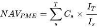
Where :
is the cashflow from the investment at date s, positive for a contribution, negative for a distribution

is the value of the index at date s

then :

Limitation
[edit]As stated in Long and Nickels paper:[1]
If a private investment greatly outperforms the index because it makes frequent, large distributions, it is possible for the final value determined by the index comparison to be negative. In effect, the frequent large withdrawals from the index result in a net short position in the index comparison
This can be simulated in the previous example by having a period where the fund distributes a large amount and the index dives :
| Period | Cashflows | Index | Index Performance | Theoretical Investment |
| p1 | -100 | 100 | 0.00% | 100 |
| p2 | -50 | 105 | 5.00% | 155 |
| p3 | 60 | 115 | 9.52% | 109.76 |
| p4 | 100 | 100 | -13.04% | -4.55 |
| Valuation (p5) | 20 | 120 | 20% | -5.47 |
| IRR | 7.77% | PME | 1.34% |
When the final valuation of the theoretical investment is negative, the IRR formula for the PME may not return any results. Even if a PME can be calculated, while the investment stays negative, every increase in the index will be interpreted as a hit in the performance of the theoretical investment : on the above example, the value of the index went back up to 120, which had a negative impact on the value of the theoretical investment. Even if the investment eventually goes back into positive values and a PME can be computed, the time spent under 0 will be improperly taken into account.[4]
The next methods by Rouvinez, and Kaplan and Schoar are partly designed to address this issue.
PME+
[edit]The PME+ was initially described in 2003 by Christophe Rouvinez[5] in a paper Private Equity Benchmarking with PME+. It is written to resolve a common issue of the Long Nickels PME : an investment outperforming the index will yield a negative value in the index theoretical investment.
PME+ Methodology
[edit]Instead of modifying the NAV of the investment, the PME+ discount every distribution by a factor computed so that the NAV of the index investment matches the NAV of the fund.
| Period | Cashflows | Index | Theoretical Contributions | Discounted Distributions | Discounted Cashflows |
| p1 | -100 | 100 | 100 | 0 | -100 |
| p2 | -50 | 105 | 50 | 0 | -50 |
| p3 | 60 | 115 | 51.63 | 51.63 | |
| p4 | 100 | 100 | 86.05 | 86.05 | |
| Valuation (p5) | 20 | 120 | 20 | ||
| Lambda | 0.86 | ||||
| IRR | 7.77% | PME+ | 2.05% |
Like the Long Nickels PME, the PME+ needs to be compared to the IRR. An IRR outperforming the PME means that the fund outperformed the public index.
PME+ Formula
[edit]Using Henly Notation in PME Benchmarking Method:[6]

where
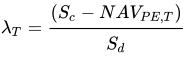
and
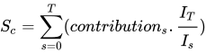
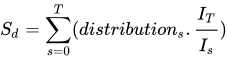
In other words, lambda is chosen so that :

The IRR is then calculated using as cashflows :

Modified PME
[edit]The modified PME (or mPME) method was released by Cambridge Associates in October 2013.[7][8] It provides an alternate way to tackle the negative NAV limitation of the LN-PME.
Like the LN-PME and the PME+, the mPME consider an hypothetical public investment whose performance follows the public benchmark. Each contribution in the private investment is matched by an equal contribution in the public investment. However, rather than subtracting the distributed amounts from the public investment, we compute the weight of the distribution in the private investment, and remove the same weight from the public one.
| Period | Call | Dist | NAV | Index | Theoretical Contributions | Distribution Weight | Theoretical NAV | Weighted Distributions | Net CF |
| p1 | 100 | 0 | 100 | 100 | 100 | 0 | 100 | 0 | -100 |
| p2 | 50 | 165 | 105 | 50 | 0 | 155 | 0 | -50 | |
| p3 | 0 | 60 | 125 | 115 | 0 | 0.32 | 114.70 | 55 | 55.06 |
| p4 | 0 | 100 | 15 | 100 | 0 | 0.87 | 13.01 | 87 | 86.73 |
| Valuation (p5) | 20 | 120 | 15.61 | 15.61 | |||||
| IRR | 7.77% | mPME | 2.02% |
Formula
[edit]For each distribution, a distribution weight is calculated
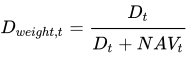
The NAV of the theoretical investment is then calculated as :

The weighted Distribution is given by :


Kaplan Schoar PME
[edit]Kaplan Schoar PME was first described in 2005 by Steve Kaplan and Antoinette Schoar.[9] While the Long Nickels PME returns an IRR, the Kaplan Schoar PME (or KS-PME) returns a market multiple. A simple explanation of its computation is described into Sorensen & Jagannathan paper:[10]
Let X(t) denote the cash flow from the fund to the LP at time t. This total cash-flow stream is divided into its positive and negative parts, called distributions (dist(t)) and capital calls (call(t)). Distributions are the cash flows returned to the LP from the PE fund (net of fees) when the fund successfully sells a company. Capital calls are the LP’s investments into the fund, including the payment of ongoing management fees. The distributions and capital calls are then valued by discounting them using the realized market returns over the same time period, and the [KS-]PME is the ratio of the two resulting values:
Formula
[edit]When considering an investment at time T. The KS-PME first considers the current valuation of the investment as a distribution at date T. KS-PME is then defined as
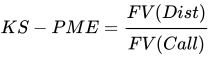
with
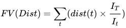
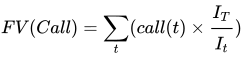
Using the previous example :
| Period | Contribution | Distribution | Index | DPI | Discounted Contribution | Discounted Distribution | KS PME | |
| p1 | 100 | 0 | 100 | 0 | 120 | 0 | 0 | |
| p2 | 50 | 0 | 105 | 0 | 57.14 | 0 | 0 | |
| p3 | 0 | 60 | 115 | 0.40 | 0 | 62.60 | 0.35 | |
| p4 | 0 | 10 | 117 | 0.47 | 0 | 10.26 | 0.41 | |
| Valuation (p5) | 0 | 110 | 120 | 1.20 | 0 | 110 | 1.03 |
While the Long Nickels PME needs to be compared to the actual IRR, the KS PME gives a direct indication of the performance of the fund compared to the performance of the index. A KS PME above 1 indicates that the fund overperformed the index. A KS PME below 1 indicates that the public index was a better investment than the fund.
Formula Simplification
[edit]The KS-PME formula can be simplified by removing from the sums :

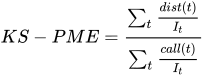
The Kaplan Schoar formula is independent of the time period used to forecast or discount the cashflows. This is an advantage over PME formulas that use an IRR calculations, whose final value will decrease over time.
Usage
[edit]The KS PME is the subject of a paper from the Columbia Business School[10] assessing that The [Kaplan Schoar] PME provides a valid economic performance measure when the investor ("LP") has log-utility preferences and the return on the LP’s total wealth equals the market return.
Relation between LN-PME and KS-PME
[edit]In a 2008 paper The common Mathematical Foundation of ACG's ICM and AICM and the K&S PME,[11] Austin Long studies the mathematical link between LN PME and KS PME.
Starting with KS PME formula :
From the LN-PME formula :
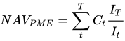


By merging the two formulas :

Direct Alpha
[edit]The Direct Alpha was introduced on March 6, 2014, in a paper by Gredil, Griffiths, and Stucke.[7]
It is deduced from the KS-PME calculation by computing an IRR using the discounted contributions and distributions, and take its natural logarithm.

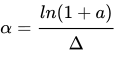
with being the time interval for which alpha is computed (usually in years)[7]

| Period | Cashflows | Index | Index Performance | Discounted Cashflows | |
| p1 | -100 | 100 | 1.20 | -120 | |
| p2 | -50 | 105 | 1.14 | -57.14 | |
| p3 | 60 | 115 | 1.04 | 62.60 | |
| p4 | 10 | 117 | 1.03 | 10.26 | |
| Valuation(p5) | 110 | 120 | 1 | 110 | |
| a (IRR) : | 1.09% | ||||
| Direct Alpha | 1.08% |
Derivation
[edit]As an introduction, it is reminded that the computation of an IRR for the set of cashflows and final value is done by solving for :


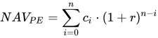
The direct alpha formula is derived from the definition of in Modern portfolio theory. We define , the rate of return, as the sum of a market return plus an alpha :


in the scope of direct alpha, we consider that r(t) and b(t) are continuous rate. Hence, the value of a cashflow at time is :



using the benchmark values, we know that :
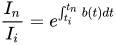
Hence :
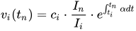
by resolving the integral, and discretizing the time variable such as :

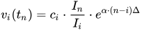
We use this formula for every contribution in the private investment :
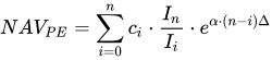
Finally, we define a as
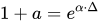
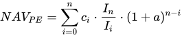
This brings us back to a typical IRR formula. In other words, the direct alpha is calculated by computing an IRR with the benchmark discounted cashflows, and then computing with
Excess IRR
[edit]Different names for this methodology includes alpha, excess IRR, Implied Private Premium ("IPP") and PME Alpha.[12][13][14]
The first reference of the alpha was in a 2005 paper from Phalippou and Gottschalg[12] and is simply named alpha, or excess IRR. The analysis is also explained in detail and named GEM Implied Private Premium (or "IPP") by Global Endowment Management[15]
Formula
[edit]The excess IRR is calculated by resolving in the following equation :

with

Methodology
[edit]To calculate the Implied Private Premium, we compute the future values of a private investment's historical distributions and contributions. Each cash flow is compounded at a rate of return equaling the benchmark's annualized return plus the IPP. We then solve for the required IPP such that the PME ratio is set to one. IPP uses annual compounding to be consistent with other reporting methodologies and comparable to IRR.
More specifically, the Implied Private Premium is solved numerically from
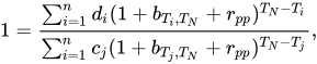
where and are contributions and distributions at time and , respectively; is the annualized benchmark return from time to , and is the IPP we are solving for.


Derivation
[edit]Starting with the definition of the IRR, which is computed by resolving in
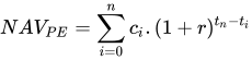
we consider r as the sum of two components : , with being the annually compounded benchmark performance between and .


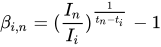

by replacing in the original equation :
Comparison with Direct Alpha
[edit]The theoretical foundation of IPP is similar to that of Direct Alpha; however, the implementation details differ. The advantage of IPP is that it's an annually compounded, arithmetic excess return. This allows IPP to be directly comparable to generally accepted performance metrics such as IRR (also an annually compounded quantity). By contrast, the continuous direct alpha is not measured in the same unit as IRR, while the discrete direct alpha is a geometric excess return.
Other PME analysis
[edit]Other less common PME analyses exists, usually as variation from either the Long Nickels PME or the Kaplan Schoar PME.
Alignment Capital defines the Alternative ICM, or AICM[11] as a variation from the Long Nickels PME :
While ACG’s ICM calculation assumes that the capital invested into the index is a long position, the alternative index comparison method (AICM) assumes the opposite – that is, the cash used to invest in the private market investment results, not from a source external to both the private market investment and the index, but from a short position in (i.e., a sale of) the index. Expressed in the same terms, the AICM calculation of the ending value of the index (the ending value used to calculate the AICM) is as follows:

In Valuing Private Equity, December 13, 2011,[16] Sorensen, Wang and Yang defines an alternate PME based on the KS PME :
There are three concerns with the standard PME measure. First, the denominator combines two types of cash flows, the investment and the management fees. Management fees are effectively a risk-free claim and should be discounted at a rate close to the risk-free rate. Second, the numerator contains the total proceeds net of carried interest. The carried interest is effectively a call option, making the LP's total payoff at maturity less risky than the underlying asset. Hence, it should be discounted at a lower rate than the underlying PE investment. Finally, the beta of the PE investment may not equal one. To address these concerns, we define the adjusted PME as follows :

![{\displaystyle Adj.PME={\cfrac {E[e^{-rT}(LP_{1}(A_{t},T)+LP_{2}(A_{T},T)+LP_{3}(A_{T},T))]}{I_{0}+E[\int _{0}^{T}e^{-rs}mX_{0}ds]}}}](https://wikimedia.org/api/rest_v1/media/math/render/svg/2b46e095b9c94b025b51407db873b6692e337b5f)
References
[edit]- ^ a b "A Private Investment Benchmark" (PDF). Retrieved 2014-03-05.
- ^ Inside Private Equity : The professional Investor Handbook by Kocis, Bachman, Long and Nickels, page 157
- ^ "Patent US7058583 - Method for calculating portfolio scaled IRR". Retrieved 2014-03-05.
- ^ Jost, Philippe; Stoll, Philipp. "Quantifying the shortness issue of PME" (PDF).
- ^ "Private Equity Benchmarking with PME+". venturecapitaljournal.com. Retrieved 2025-08-15.
- ^ Samuel Henly (2013-08-12). "PME Benchmarking Methods" (PDF). Retrieved 2014-03-05.
- ^ a b c "Benchmarking Private Equity: The Direct Alpha Method". SSRN 2403521.
{{cite journal}}: Cite journal requires|journal=(help) - ^ "New Method for Comparing Performance of Private Investments with Public Investments Introduced by Cambridge Associates". Cambridge Associates.
- ^ "Private Equity Performance:Returns, Persistence and Capital Flows" (PDF). University of Chicago Graduate School of Business. Retrieved 2014-03-05.
- ^ a b Morten Sorensen, Ravi Jagannathan. "The Public Market Equivalent and Private Equity Performance". Papers.ssrn.com. SSRN 2347972.
{{cite journal}}: Cite journal requires|journal=(help) - ^ a b "A Method for Quantifying Concentration of Returns in Private Equity Portfolios" (PDF). Retrieved 2014-03-05.
- ^ a b "Performance of Private Equity Funds, page 17". Ludovic Phalippou & Olivier Gottschalg. SSRN 473221.
{{cite journal}}: Cite journal requires|journal=(help) - ^ "Evolution of MIRR: PME Alpha". Retrieved 11 December 2014.
{{cite web}}: CS1 maint: deprecated archival service (link) - ^ "The GEM Implied Private Premium (IPP) Private Equity Benchmark" (PDF). Global Endowment Management, LP. Retrieved 2014-11-21.
- ^ "Trademark GEM implied Private Premium".
- ^ "Valuing private equity" (PDF). 2011-12-13. Retrieved 2014-03-05.
- Exposed to the J-Curve: Understanding and Managing Private Equity Fund Investments, Ulrich Grabenwarter & Tom Weidig, Chapter 5

Public Market Equivalent
View on GrokipediaOverview
Definition and Purpose
The Public Market Equivalent (PME) is a performance measurement tool used to benchmark private equity and venture capital fund returns against a public market index by replicating the fund's cash flow pattern in a hypothetical public investment portfolio.[6] This approach yields a ratio where a value greater than 1 signifies outperformance relative to the public benchmark, while a value less than 1 indicates underperformance.[7] The original form, known as the Long-Nickels PME, adjusts contributions and distributions from the private fund by the corresponding returns of the selected public index to compute this ratio.[6] The primary purpose of PME is to overcome the limitations of the Internal Rate of Return (IRR), which ignores the time value of money in relation to public market opportunities and can overstate performance for illiquid investments like private equity and venture capital due to its sensitivity to cash flow timing assumptions.[8] By incorporating the opportunity cost of committing capital to private markets instead of liquid public alternatives, PME enables investors to assess whether private funds generate excess returns that justify their illiquidity, higher fees, and longer lock-up periods.[9] This makes it particularly valuable for institutional investors evaluating alternative asset allocations in diversified portfolios.[10] PME emerged in the late 1990s as a standardized method for comparing private investments to public markets, coinciding with the significant expansion of private equity assets under management from approximately $600 billion in 2000 to $1.7 trillion by 2010.[6][11][12] This growth underscored the need for robust benchmarking to quantify the relative merits of private markets amid increasing institutional adoption.[13]Historical Development
The Public Market Equivalent (PME) methodology originated in the mid-1990s as a tool to benchmark private equity performance against public markets, addressing the challenges of illiquidity and irregular cash flows in traditional metrics like internal rate of return (IRR). The foundational approach, known as the Long-Nickels PME or Index Comparison Method (ICM), was introduced by Austin M. Long III and Craig J. Nickels in their 1996 working paper "A Private Investment Benchmark." This method simulates a hypothetical public market investment mirroring the timing and magnitude of private fund cash flows, typically using indices like the S&P 500 to evaluate relative performance.[1] Early applications focused on simplifying comparisons for institutional investors, establishing PME as a practical alternative to IRR for assessing value creation beyond market returns.[14] In 2005, Steven N. Kaplan and Antoinette Schoar proposed a simplified variant in their seminal paper "Private Equity Performance: Returns, Persistence, and Capital Flows," published in the Journal of Finance. The Kaplan-Schoar PME calculates a ratio of the present value of private equity distributions to contributions, discounted at public market rates, providing a multiple-based measure that avoids IRR's sensitivity to cash flow timing. This adaptation gained traction for its computational ease and ability to handle multi-period cash flows more robustly, influencing academic and practitioner analyses of private equity persistence and capital flows.[2] Refinements continued in the early 2000s to address limitations in handling early distributions and follow-on investments. In 2003, Christophe Rouvinez introduced PME+ in the article "Private Equity Benchmarking with PME+" published in Venture Capital Journal, incorporating a scaling factor to adjust distributions and prevent negative public portfolio values, thereby better accommodating funds with premature exits or additional capital calls.[15] Later, in 2013, Cambridge Associates developed the Modified PME (mPME) to further enhance multi-period accuracy by dynamically scaling cash flows, reducing approximation errors in long-term benchmarks.[16] By the 2010s, PME methodologies saw widespread adoption for standardized reporting in private equity, with industry bodies like the Institutional Limited Partners Association (ILPA) promoting their use in guidelines such as the 2017 white paper on policy benchmark selection to improve transparency and comparability across funds.[17] As of 2025, PME remains a core metric in regulatory filings and investor due diligence, with ongoing refinements to address emerging challenges like ESG integration and market volatility.[18]Core Concepts
Public Market Index Selection
The selection of a public market index is a critical step in calculating the Public Market Equivalent (PME), as it establishes the benchmark against which private fund performance is evaluated. The primary criterion is relevance to the fund's investment strategy, ensuring the index mirrors the geographic focus, market capitalization, and sector exposure of the underlying investments. For instance, venture capital funds targeting small-cap U.S. companies often use the Russell 2000 Index, while global private equity portfolios may benchmark against the MSCI World Index to capture broad international equity exposure. Additionally, the index must provide comprehensive total return data, incorporating dividends and capital gains, to accurately reflect reinvestment opportunities comparable to private fund cash flows.[19][14] Common indices employed in PME analyses include the S&P 500 for U.S. large-cap strategies, the FTSE 100 for UK-focused funds, and the NASDAQ Composite for technology-oriented investments. These selections align with the fund's profile; for example, buyout funds frequently reference the Russell 3000 to encompass a wider U.S. equity universe, while European private equity may utilize the MSCI Europe Index. Such indices are favored due to their established track records and alignment with private market dynamics, providing a standardized public counterpart for performance attribution.[19][20] Key considerations in index selection include data frequency, currency alignment, and mitigation of biases. Monthly return data is typically preferred for practicality in matching irregular private cash flows, though daily data may be used for precision in shorter horizons. Currency matching ensures comparability, with indices denominated in the fund's base currency—such as USD for North American funds or EUR for Eurozone investments—to avoid exchange rate distortions. To address survivorship bias, where historical index performance may overstate returns by excluding failed companies, analysts select well-constructed, market-cap-weighted indices like the S&P 500 or MSCI World, which incorporate adjustments for delistings and maintain comprehensive coverage of the equity universe. These factors collectively ensure the index serves as a reliable prerequisite for cash flow discounting across PME variants.[19][14]Cash Flow Timing and Discounting
In the Public Market Equivalent (PME) framework, cash flows from private investments are timed precisely to reflect the investor's perspective, where capital calls represent outflows (negative cash flows) requiring investment into the fund, and distributions represent inflows (positive cash flows) returned to the investor.[7] These cash flows are typically dated to the exact occurrence, often at a monthly granularity or finer, such as specific days, to capture the irregular pacing of private equity commitments and realizations.[21] At the fund's liquidation or valuation date, any residual net asset value (NAV) is treated as a final positive cash flow, simulating a complete distribution of remaining assets to the investor.[22] The discounting process in PME replicates the private cash flows within a public market benchmark by applying the index's returns to mimic the timing and magnitude of investments and withdrawals. For each capital call, an equivalent amount is notionally invested in the public index (such as the S&P 500) on the call date, accruing returns until a corresponding distribution date or the terminal period.[21] Distributions are then replicated by withdrawing the specified amounts from the accumulated public portfolio on their respective dates, with any remaining balance carried forward to accumulate a net present value or terminal value that can be compared to the private fund's performance.[7] This replication accounts for the opportunity cost of capital by using realized public market returns over the exact holding periods dictated by the private cash flow schedule.[22] To handle timing irregularities, such as cash flows occurring on non-month-end dates when public indices provide only periodic data, linear interpolation is commonly applied to estimate intermediate index returns, ensuring accurate accrual from the precise cash flow dates.[21] The residual NAV at the analysis endpoint serves as the terminal value in this replication, effectively closing out the hypothetical public portfolio and allowing for a comprehensive assessment of relative performance without assuming ongoing fund operations.[19]Long-Nickels PME
Methodology
The Long-Nickels PME methodology, originally developed as the Index Comparison Method (ICM) in 1996, provides a benchmark for private equity performance by replicating the fund's cash flow timing in a public market index, such as the S&P 500, and computing an equivalent public IRR for direct comparison.[1][23] The step-by-step process begins with selecting an appropriate public market index, such as the S&P 500, as input for generating returns. Hypothetical public cash flows are then created to mirror the timing of the private fund's contributions (as outflows) and distributions (as inflows), with the index returns applied to adjust these flows for the periods between cash flow dates. The internal rate of return (IRR) for these public cash flows is computed, providing an effective public benchmark IRR that accounts for the irregular timing of private equity investments. This public IRR is compared to the private fund's IRR to determine relative performance, where a higher private IRR indicates outperformance.[1][14] This IRR-focused equivalence emphasizes computational ease, as it avoids the complexities of multi-period compounding or terminal value adjustments beyond the cash flow replication, enabling a straightforward assessment of whether the private investment generated excess returns over the public equivalent.[1]Formula
The Long-Nickels Public Market Equivalent (LN-PME) involves computing the public market IRR () by solving for the discount rate $ r $ that equates the net present value of the adjusted public cash flows to zero:Limitations
The Long-Nickels Public Market Equivalent (PME) is highly sensitive to the precise timing of cash flows, as even minor shifts in dates—such as a few days—can significantly alter outcomes due to the volatility of public market returns.[14] This sensitivity arises because the method replicates private equity cash flows by investing in a public index at exact call dates and withdrawing at distribution dates, amplifying the impact of short-term market fluctuations on the calculated net present value.[23] A key shortcoming is the method's inability to handle early fund liquidations properly, which occurs when a private equity fund distributes all capital before the public index replication reaches a terminal value, leading to negative or undefined net asset values in approximately 5-6.4% of cases and rendering the PME incalculable for about one in 16 funds.[24] Similarly, the approach overlooks the distinct risk profile of follow-on investments, where additional capital is deployed into existing portfolio companies rather than new opportunities, potentially overstating performance by treating all capital calls as equivalent public market investments without adjusting for concentrated exposure.[25] These omissions can bias results upward, as the hypothetical public portfolio assumes diversified reinvestment that does not mirror private equity's illiquid, lumpy commitments. The Long-Nickels PME assumes a perfect replication of private equity's leverage and fee structure in public markets, which is unrealistic since public indices typically reflect unlevered, gross-of-fee returns while private funds employ significant debt and incur management expenses that reduce net performance.[14] This mismatch implies a beta of 1.0 relative to the benchmark, ignoring the higher systematic risk and costs inherent in private equity, leading to distorted comparisons that understate the challenges of achieving equivalent risk-adjusted outcomes.[25] Empirically, studies have shown that the Long-Nickels PME often exceeds 1.0—even for underperforming private equity funds—during bull markets, as elevated public returns inflate the benchmark despite mediocre or negative private internal rates of return.[25] For instance, analyses of buyout funds reveal a downward bias in median PME estimates compared to alternative measures like direct alpha, highlighting how market conditions can mask true underperformance.[25] These issues have prompted developments like the PME+ variant to mitigate timing and liquidation sensitivities.[26] While PME provides a robust relative benchmark accounting for cash flow timing and opportunity cost, it can be noisy for individual funds due to volatility in private cash flows. Simulations show higher standard deviation in PME estimates compared to newer methods. A recent advancement is the α metric proposed by Arthur Korteweg and Stefan Nagel (2024), which constructs a benchmark removing common factor shocks and systematic risk more precisely, yielding less noisy fund-level abnormal returns than PME or Generalized PME (GPME). α matches GPME's aggregate implications but improves accuracy for individual fund evaluation and persistence analysis.[27] Institutional investors often complement PME with beta adjustments (estimating PE's market exposure, typically 1.0-1.3 for buyouts), de-smoothing techniques to correct for understated volatility in reported returns, and portfolio-level considerations like diversification benefits and illiquidity premia.PME+
Methodology
PME+ is a variant of the Public Market Equivalent (PME) methodology developed by Christophe Rouvinez at Capital Dynamics in 2003 to address limitations in the original Long-Nickels PME, particularly the potential for negative net asset values (NAVs) in the public benchmark portfolio when private equity significantly outperforms the public index.[15] The process begins with selecting a public market index, such as the S&P 500. The private fund's capital contributions (outflows) and distributions (inflows) are replicated in the public index by investing contributions upon receipt and liquidating portions of the public portfolio to match distributions. Unlike the standard PME, which may result in a negative terminal public NAV if cumulative distributions exceed the grown contributions, PME+ introduces a scaling factor λ applied to all distributions. This factor ensures the terminal value of the public portfolio equals the private fund's terminal NAV, maintaining a positive NAV throughout and providing a more realistic benchmark without implied short-selling. The performance is then measured as the internal rate of return (IRR) of these adjusted public cash flows, compared to the private fund's IRR. A higher private IRR indicates outperformance.[22] This adjustment preserves the timing of cash flows while eliminating anomalies from extreme outperformance, making PME+ suitable for evaluating illiquidity premiums in private equity.[22]Formula
The PME+ is calculated as the IRR of the adjusted public market cash flows:Modified PME
Methodology
The Modified Public Market Equivalent (mPME), developed by Cambridge Associates in 2013, is a proprietary benchmarking method for private equity and venture capital funds that refines earlier PME approaches by addressing issues such as negative net asset values (NAV) in the public equivalent portfolio, particularly during periods of underperformance or volatility.[14] Unlike the Kaplan-Schoar PME, which uses direct present or future value ratios, mPME simulates the private fund's cash flows in a public market index while ensuring the public portfolio remains non-negative.[28] The process starts with selecting a public market index, such as the S&P 500 or Russell 2000, to represent the benchmark. Private fund contributions (capital calls) are treated as investments into the public index at the time they occur, growing at the index's returns until subsequent events. For distributions (realizations), the public equivalent withdrawal is scaled by the ratio of the private distribution amount to the private fund's current NAV (or remaining invested capital). This scaling caps the public distribution at the available public portfolio value, preventing negative balances that could arise if private distributions exceed the hypothetical public growth. Any excess private distribution beyond the public capacity is set to zero in the public simulation. This adjusted public cash flow series then allows computation of performance metrics like internal rate of return (IRR), distributions to paid-in capital (DPI), and total value to paid-in capital (TVPI) for direct comparison to the private fund's metrics. A public IRR or multiple exceeding the private equivalent indicates underperformance relative to the benchmark.[14] This method emphasizes realism in replication, avoiding distortions from uncapped withdrawals, and has been widely adopted in limited partner (LP) reporting and fund evaluations as of 2025, particularly for vintages post-Global Financial Crisis where market volatility highlights its advantages.[29]Formula
The mPME does not use a single closed-form ratio like some PME variants; instead, it generates adjusted public cash flows for metric calculation. Let $ C_t $ be private contributions at time $ t $, $ D_t $ private distributions at time $ t $, $ NAV_t $ the private fund's NAV just before $ D_t $, and $ P_u $ the public index value at time $ u $. Public contributions are $ PublicC_t = C_t $. The public portfolio value before distribution at $ t $ is the prior value grown by index returns: $ PublicNAV_t = PublicNAV_{t-1} \times \frac{P_t}{P_{t-1}} + PublicC_t \times \frac{P_t}{P_t} $ (simplified, assuming discrete periods). The public distribution is then $ PublicD_t = \min\left( D_t \times \frac{PublicNAV_t}{NAV_t + C_t - D_t}, PublicNAV_t \right) $, ensuring proportionality and non-negativity. The updated public NAV after distribution is $ PublicNAV_t = PublicNAV_t - PublicD_t $. The public IRR is solved as the $ r $ where $ \sum_t \frac{PublicCF_t}{(1 + r)^{t}} = 0 $, with $ PublicCF_t = -PublicC_t + PublicD_t $. Performance is assessed by comparing this public IRR (or DPI/TVPI from public flows) to private metrics; mPME outperformance occurs when private > public. Numerical methods (e.g., Newton-Raphson) are used for IRR, and the approach preserves timing without terminal value assumptions beyond final NAV if needed.[14][28]Kaplan-Schoar PME
Methodology
The Kaplan-Schoar PME methodology calculates private equity fund performance relative to a public market benchmark by determining the ratio of the present value of the fund's distributions to the present value of its contributions, with all cash flows discounted using the returns from a selected public market index, such as the S&P 500. This approach simulates the outcome of investing the same cash flows in the public index, providing a direct measure of whether the private fund outperformed the public alternative after accounting for timing and illiquidity.[2] The process begins with selecting an appropriate public market index to generate the discount factors based on its historical total returns. For each private fund contribution (capital call, treated as an outflow) at time $ t $, the present value is computed by dividing the amount by the cumulative index return from time 0 to $ t $. Similarly, each distribution (capital return, treated as an inflow) at time $ u $ is discounted by the cumulative index return from time 0 to $ u $. If the fund has a residual net asset value (NAV) at the evaluation date, it is included as a final distribution. The KS-PME is then the ratio of the sum of discounted distributions (including NAV) to the sum of discounted contributions. A ratio greater than 1 indicates that the private fund generated excess returns relative to the public benchmark.[2] This method emphasizes simplicity and economic intuition, as it directly incorporates public market returns as the discount rate without assuming constant reinvestment or requiring iterative solutions, while adjusting for the irregular timing of private equity cash flows.[2]Formula
The Kaplan-Schoar Public Market Equivalent (KS-PME) is defined as the ratio of the present value of distributions to the present value of contributions, discounted using the public market index returns:Relation to Long-Nickels PME
The Kaplan-Schoar PME (KS-PME) and Long-Nickels PME (LN-PME) share a common mathematical foundation rooted in the terminal value of a public market index replicating private equity cash flows, allowing for conceptual and approximate equivalence under specific assumptions.[30] Introduced by Long and Nickels in 1996 as the Index Comparison Method (ICM), the LN-PME computes an internal rate of return (IRR) for a hypothetical public portfolio mirroring private contributions and distributions, while the KS-PME, developed by Kaplan and Schoar in 2005, yields a multiple comparing the future value of distributions (plus net asset value) to contributions, both compounded at public index returns.[21][2] Under continuous compounding and log-normal distribution of public returns, the KS-PME approximates the LN-PME, as the multiple can be converted to an IRR via $ r \approx \frac{\ln(\text{KS-PME})}{\text{duration}} $, linking the geometric mean return implicit in the LN-PME's IRR solution to the exponential form of the KS multiple.[30] A derivation sketch reveals this connection through the terminal index value: for LN-PME, the ending value balances invested and returned capital as $ \text{Ending Value} = \text{FV}{\text{Invested}} - \text{FV}{\text{Returned}} $, while KS-PME expresses the ratio as $ \text{PME} = 1 - \frac{\text{Ending Value}}{\text{FV}_{\text{Invested}}} $, enabling translation between the IRR and multiple when returns are continuously compounded and log-normally distributed.[30] In practice, the KS-PME is computationally simpler and always defined, avoiding IRR solvability issues in LN-PME (such as negative net asset values in 5-10% of cases from early distributions), though it assumes uniform compounding and can undervalue timing effects in discrete flows where LN-PME provides greater precision.[25][19] Empirical studies demonstrate high alignment between the two, with correlation coefficients often exceeding 0.9 across private equity datasets, reflecting their shared reliance on public market replication despite output differences (e.g., IRR spreads vs. multiples greater than 1 indicating outperformance).[25]Other Variants
Direct Alpha
Direct Alpha is a performance measurement variant within the Public Market Equivalent framework that decomposes private equity returns into an alpha component, representing skill-based excess returns independent of market exposure, and a beta component, capturing systematic risk relative to a public market benchmark. Introduced to address limitations in traditional internal rate of return (IRR) comparisons, such as sensitivity to cash flow timing and reinvestment assumptions, Direct Alpha provides a risk-adjusted excess return metric suitable for illiquid investments.[31][25] The methodology constructs hypothetical value time series from observed cash flows for both private and public portfolios, then applies a log-linear regression to estimate parameters without relying on unobserved net asset values (NAVs). For the public portfolio, the value at each time is computed by replicating the private cash flow timings: contributions are invested in the public index, growing at public market returns until distributions are withdrawn, yielding a series that mirrors the benchmark exposure of the private investment. The private value series is similarly derived but assumes reinvestment of cash flows at a constant rate consistent with the model's log-return dynamics, enabling the regression analysis. This regression takes the form:Excess IRR
The Excess IRR, also known as excess return or Implied Private Premium (IPP) in some contexts, serves as a straightforward variant of the Public Market Equivalent (PME) methodology to evaluate private equity fund performance by directly measuring the outperformance relative to a public market benchmark. It gauges the additional return generated by the private fund beyond what would have been achieved by investing the same cash flows in a public equity index, thereby addressing the timing mismatch inherent in illiquid private investments. This approach assumes that the private fund's cash flow schedule—encompassing contributions, distributions, and the residual value—can be replicated in the public market to provide a like-for-like comparison, highlighting the value added (or subtracted) by private equity managers after accounting for market exposure and liquidity differences.[34] The methodology involves two primary steps: first, calculating the internal rate of return (IRR) for the private equity fund based on its actual cash flows, which include investor contributions (outflows), distributions (inflows), and any terminal value at the fund's end. Second, computing a public market IRR by simulating a public portfolio that replicates the private cash flow timings: contributions are invested in a chosen public equity benchmark, such as the S&P 500 or Nasdaq Composite, upon drawdown, with the portfolio growing at index returns, and a proportional fraction liquidated at each distribution date to match the private distributions. This public IRR reflects the opportunity cost of capital tied up in the private fund over the same irregular intervals, enabling a risk-adjusted assessment without requiring complex discounting or regression adjustments. For instance, in analyses of mature funds from 1981 to 1993, this method revealed average private IRRs of approximately 19.81%, compared to public IRRs of 14.1% using the S&P 500 with matched timing, underscoring the importance of cash flow synchronization.[34] The formula for Excess IRR is derived from the fundamental concept of return differential, where the private fund's compounded growth rate is subtracted from the benchmark's equivalent rate, assuming both are exposed to similar market risks but differing in liquidity and selection timing; note that this difference approximates the excess return but may be affected by differing reinvestment assumptions in IRR calculations:Comparisons and Applications
Comparison of PME Variants
The Long-Nickels PME (LN-PME) and PME+ variants differ primarily in their treatment of cash distributions and residual values, with PME+ incorporating a scaling factor to align the hypothetical public portfolio's net asset value (NAV) with the private fund's at exit, thereby better accommodating follow-on investments and reinvestments common in private equity structures.[35][22] In contrast, the Kaplan-Schoar PME (KS-PME) offers computational simplicity by producing a single ratio of total wealth multiples rather than an IRR, trading some precision in annualized return measurement for ease of calculation and robustness across datasets, while LN-PME provides a more precise IRR-based output but requires iterative solving that can fail in cases of extreme distributions.[23][36] Direct Alpha isolates manager skill by calculating the IRR of benchmark-compounded cash flows, emphasizing alpha generation independent of timing, whereas Excess IRR simply subtracts the benchmark IRR from the private IRR, offering a straightforward differential but failing to disentangle skill from market exposure.[31][22]| Variant Pair | Key Differences in Assumptions and Outputs | Suitability |
|---|---|---|
| LN-PME vs. PME+ | LN-PME assumes direct cash flow replication in the benchmark, yielding an IRR spread; PME+ scales distributions by a fixed factor (often 1.0 for inflows) to match NAVs, producing an adjusted IRR that better reflects liquidation scenarios. | PME+ suits funds with significant follow-ons or uneven distributions; LN-PME is simpler for basic benchmarking but can undervalue residuals.[35][22] |
| KS-PME vs. LN-PME | KS-PME assumes a wealth multiple comparison without rate assumptions; LN-PME derives an investable IRR from replicated flows. | KS-PME excels in computational ease for large-scale analysis; LN-PME offers precision for rate-focused evaluations but is more error-prone.[23][36] |
| Direct Alpha vs. Excess IRR | Direct Alpha assumes benchmark compounding to a common horizon for alpha isolation; Excess IRR assumes direct subtraction of IRRs without timing adjustments. | Direct Alpha better isolates skill in volatile markets; Excess IRR provides a simple proxy but conflates beta and alpha.[31][22] |