RL circuit
RL circuit
Main page

RL circuit

logo
Community Hub0 subscribers
Read side by side
from Wikipedia

A resistor–inductor circuit (RL circuit), or RL filter or RL network, is an electric circuit composed of resistors and inductors driven by a voltage or current source.[1] A first-order RL circuit is composed of one resistor and one inductor, either in series driven by a voltage source or in parallel driven by a current source. It is one of the simplest analogue infinite impulse response electronic filters.

Introduction

[edit]

The fundamental passive linear circuit elements are the resistor (R), capacitor (C) and inductor (L). They can be combined to form the RC circuit, the RL circuit, the LC circuit and the RLC circuit, with the abbreviations indicating which components are used. These circuits exhibit important types of behaviour that are fundamental to analogue electronics. In particular, they are able to act as passive filters.

Capacitors are usually preferred to inductors since they can be more easily manufactured and are generally physically smaller, particularly for higher values of components. But parasitic inductance may still be unavoidable.

Both RC and RL circuits form a single-pole filter. Depending on whether the reactive element (C or L) is in series with the load, or parallel with the load will dictate whether the filter is low-pass or high-pass.

Frequently RL circuits are used as DC power supplies for RF amplifiers, where the inductor is used to pass DC bias current and block the RF getting back into the power supply.

Complex impedance

[edit]

The complex impedance ZL (in ohms) of an inductor with inductance L (in henries) is

The complex frequency s is a complex number,

where

Eigenfunctions

[edit]

The complex-valued eigenfunctions of any linear time-invariant (LTI) system are of the following forms:
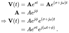
From Euler's formula, the real-part of these eigenfunctions are exponentially-decaying sinusoids:

Sinusoidal steady state

[edit]

Sinusoidal steady state is a special case in which the input voltage consists of a pure sinusoid (with no exponential decay). As a result,

and the evaluation of s becomes

Series circuit

[edit]
Series RL circuit

By viewing the circuit as a voltage divider, we see that the voltage across the inductor is:
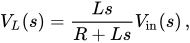
and the voltage across the resistor is:
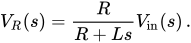
Current

[edit]

The current in the circuit is the same everywhere since the circuit is in series:
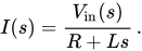
Transfer functions

[edit]

The transfer function to the inductor voltage is

Similarly, the transfer function to the resistor voltage is

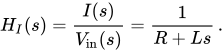
The transfer function, to the current, is
Poles and zeros

[edit]

The transfer functions have a single pole located at

In addition, the transfer function for the inductor has a zero located at the origin.

Gain and phase angle

[edit]

The gains across the two components are found by taking the magnitudes of the above expressions:

and

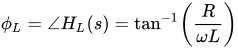
and the phase angles are:
and

Phasor notation

[edit]

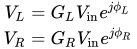
These expressions together may be substituted into the usual expression for the phasor representing the output:[2]
Impulse response

[edit]

The impulse response for each voltage is the inverse Laplace transform of the corresponding transfer function. It represents the response of the circuit to an input voltage consisting of an impulse or Dirac delta function.

The impulse response for the inductor voltage is

where u(t) is the Heaviside step function and τ = L/R is the time constant.

Similarly, the impulse response for the resistor voltage is

Zero-input response

[edit]

The zero-input response (ZIR), also called the natural response, of an RL circuit describes the behavior of the circuit after it has reached constant voltages and currents and is disconnected from any power source. It is called the zero-input response because it requires no input.

The ZIR of an RL circuit is:

Frequency domain considerations

[edit]

These are frequency domain expressions. Analysis of them will show which frequencies the circuits (or filters) pass and reject. This analysis rests on a consideration of what happens to these gains as the frequency becomes very large and very small.

As ω → ∞:

As ω → 0:

This shows that, if the output is taken across the inductor, high frequencies are passed and low frequencies are attenuated (rejected). Thus, the circuit behaves as a high-pass filter. If, though, the output is taken across the resistor, high frequencies are rejected and low frequencies are passed. In this configuration, the circuit behaves as a low-pass filter. Compare this with the behaviour of the resistor output in an RC circuit, where the reverse is the case.

The range of frequencies that the filter passes is called its bandwidth. The point at which the filter attenuates the signal to half its unfiltered power is termed its cutoff frequency. This requires that the gain of the circuit be reduced to
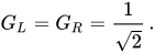
Solving the above equation yields

which is the frequency that the filter will attenuate to half its original power.

Clearly, the phases also depend on frequency, although this effect is less interesting generally than the gain variations.

As ω → 0:

As ω → ∞:

So at DC (0 Hz), the resistor voltage is in phase with the signal voltage while the inductor voltage leads it by 90°. As frequency increases, the resistor voltage comes to have a 90° lag relative to the signal and the inductor voltage comes to be in-phase with the signal.

Time domain considerations

[edit]
This section relies on knowledge of e, the natural logarithmic constant.

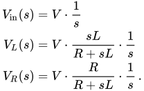
The most straightforward way to derive the time domain behaviour is to use the Laplace transforms of the expressions for VL and VR given above. This effectively transforms s. Assuming a step input (i.e., Vin = 0 before t = 0 and then Vin = V afterwards):
Inductor voltage step-response.
Resistor voltage step-response.

Partial fractions expansions and the inverse Laplace transform yield:
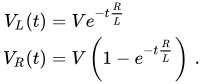
Thus, the voltage across the inductor tends towards 0 as time passes, while the voltage across the resistor tends towards V, as shown in the figures. This is in keeping with the intuitive point that the inductor will only have a voltage across as long as the current in the circuit is changing — as the circuit reaches its steady-state, there is no further current change and ultimately no inductor voltage.

These equations show that a series RL circuit has a time constant, usually denoted τ = L/R being the time it takes the voltage across the component to either fall (across the inductor) or rise (across the resistor) to within 1/e of its final value. That is, τ is the time it takes VL to reach V(1/e) and VR to reach V(1 − 1/e).

The rate of change is a fractional 1 − 1/e per τ. Thus, in going from t = to t = (N + 1)τ, the voltage will have moved about 63% of the way from its level at t = toward its final value. So the voltage across the inductor will have dropped to about 37% after τ, and essentially to zero (0.7%) after about 5τ. Kirchhoff's voltage law implies that the voltage across the resistor will rise at the same rate. When the voltage source is then replaced with a short circuit, the voltage across the resistor drops exponentially with t from V towards 0. The resistor will be discharged to about 37% after τ, and essentially fully discharged (0.7%) after about 5τ. Note that the current, I, in the circuit behaves as the voltage across the resistor does, via Ohm's law.

The delay in the rise or fall time of the circuit is in this case caused by the back-EMF from the inductor which, as the current flowing through it tries to change, prevents the current (and hence the voltage across the resistor) from rising or falling much faster than the time-constant of the circuit. Since all wires have some self-inductance and resistance, all circuits have a time constant. As a result, when the power supply is switched on, the current does not instantaneously reach its steady-state value, V/R. The rise instead takes several time-constants to complete. If this were not the case, and the current were to reach steady-state immediately, extremely strong inductive electric fields would be generated by the sharp change in the magnetic field — this would lead to breakdown of the air in the circuit and electric arcing, probably damaging components (and users).

These results may also be derived by solving the differential equation describing the circuit:
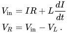
The first equation is solved by using an integrating factor and yields the current which must be differentiated to give VL; the second equation is straightforward. The solutions are exactly the same as those obtained via Laplace transforms.

Short circuit equation

[edit]

For short circuit evaluation, RL circuit is considered. The more general equation is:

With initial condition:

Which can be solved by Laplace transform:

Thus:
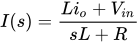
Then inverse Laplace transform will then take the form:

where is the response from the initial current at , is the transient response of the circuit, and is the steady-state response. For all inputs, the inverse transfer takes the form:

Where the inverse Laplace transform represents the transient and steady-state responses, based on different inputs. In case the source voltage is a Heaviside step function (DC):
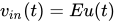
the transform returns:

where is the transient response and the steady-state response.

In case the source voltage is a sinusoidal function (AC):

the transformer returns:

Mathematically, this transformer proves complex, however it takes the same basic form as with the Heaviside step function:

Where and and the magnitude and phase-shift of :

and

Returning:

can then be solved using information about the initial conditions. In this example, at , reducing the equation to:

Making the final equation:

Parallel circuit

[edit]
Parallel RL circuit

When both the resistor and the inductor are connected in parallel connection and supplied through a voltage source, this is known as a RL parallel circuit.[2] The parallel RL circuit is generally of less interest than the series circuit unless fed by a current source. This is largely because the output voltage (Vout) is equal to the input voltage (Vin); as a result, this circuit does not act as a filter for a voltage input signal.

With complex impedances:
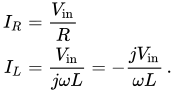
This shows that the inductor lags the resistor (and source) current by 90°.

The parallel circuit is seen on the output of many amplifier circuits, and is used to isolate the amplifier from capacitive loading effects at high frequencies. Because of the phase shift introduced by capacitance, some amplifiers become unstable at very high frequencies, and tend to oscillate. This affects sound quality and component life, especially the transistors.

See also

[edit]

References

[edit]
Revisions and contributorsEdit on WikipediaRead on Wikipedia
from Grokipedia
An RL circuit is an electrical circuit composed of a resistor and an inductor connected in series or parallel, driven by a voltage or current source, and is fundamental for analyzing transient and steady-state behaviors in electrical engineering.[1] The resistor limits current flow and dissipates energy as heat, while the inductor stores energy in a magnetic field and opposes changes in current through induced voltage.[2] In direct current (DC) applications, the circuit exhibits transient responses where current grows or decays exponentially after a switch event, characterized by a time constant τ=L/R\tau = L/R, where LL is inductance in henries and RR is resistance in ohms; after approximately five time constants, the circuit reaches steady state with the inductor behaving as a short circuit.[3] The current in such transients follows i(t)=I()+[i(0+)I()]et/τi(t) = I(\infty) + [i(0^+) - I(\infty)] e^{-t/\tau}, where i(0+)i(0^+) is the initial current and I()I(\infty) is the final steady-state current.[4] In alternating current (AC) scenarios, the inductor introduces reactance XL=2πfLX_L = 2\pi f L, where ff is frequency, resulting in an impedance Z=R2+XL2Z = \sqrt{R^2 + X_L^2} for series configurations and a phase difference where voltage leads current by θ=tan1(XL/R)\theta = \tan^{-1}(X_L / R).[5] RL circuits are essential in applications such as filters, where series configurations act as low-pass filters attenuating high frequencies, and in power electronics for managing current surges and energy storage.[1]

Fundamentals

Components and Configuration

An RL circuit is an electrical circuit composed of a resistor (R) and an inductor (L), typically connected to a voltage or current source.[6] The resistor limits the flow of electric current and dissipates electrical energy as heat according to Ohm's law, which states that the voltage drop across the resistor is $ V_R = I R $, where $ I $ is the current and $ R $ is the resistance.[7] The inductor, often a coil of wire, stores energy in a magnetic field and opposes changes in current; its voltage is given by Faraday's law of induction as $ V_L = L \frac{dI}{dt} $, where $ L $ is the inductance.[8] Resistance is measured in ohms ($ \Omega $), while inductance is measured in henries (H).[6] A key property of inductors is that current through them cannot change instantaneously, so the current immediately before and after a switching event remains the same: $ i(0^-) = i(0^+) $.[9] Standard configurations include the series RL circuit, where the resistor and inductor share the same current in a single path connected to a voltage source, such that the total voltage is the sum of the drops across each component (as in a loop diagram with source, R, and L in sequence).[6] In the parallel RL circuit, the resistor and inductor share the same voltage across them from the source, with currents adding up through each branch (as in a diagram with source connected to both R and L in parallel branches).[9] The ratio $ \tau = L/R $ serves as a characteristic time constant for the circuit's response.[6]

Basic Equations

In a series RL circuit, the fundamental equation is derived from Kirchhoff's voltage law (KVL), which states that the supplied voltage equals the sum of the voltage drops across the resistor and inductor. The voltage across the resistor is $ Ri(t) $, and across the inductor is $ L \frac{di(t)}{dt} $, yielding
Vs(t)=Ri(t)+Ldi(t)dt. V_s(t) = R i(t) + L \frac{di(t)}{dt}.
This equation reflects the inductor's property that its voltage opposes changes in current, consistent with Lenz's law.[10] Rearranging the KVL equation produces the standard first-order linear differential equation for the current:
di(t)dt+RLi(t)=1LVs(t). \frac{di(t)}{dt} + \frac{R}{L} i(t) = \frac{1}{L} V_s(t).
The general solution to this differential equation consists of the homogeneous solution plus a particular solution. The homogeneous equation dih(t)dt+RLih(t)=0\frac{di_h(t)}{dt} + \frac{R}{L} i_h(t) = 0 has the solution ih(t)=Ae(R/L)ti_h(t) = A e^{-(R/L)t}, where AA is a constant determined by initial conditions and τ=L/R\tau = L/R is the time constant. The particular solution ip(t)i_p(t) depends on the form of the source voltage Vs(t)V_s(t); for a constant input, ip(t)=Vs/Ri_p(t) = V_s / R, while for an exponential input Vs(t)=V0estV_s(t) = V_0 e^{st}, assume ip(t)=Kesti_p(t) = K e^{st} and solve for KK.[11][10] For a parallel RL circuit driven by a current source, Kirchhoff's current law (KCL) at the common node equates the source current to the sum of the resistor and inductor branch currents. The resistor current is V(t)/RV(t)/R, and the inductor current is (1/L)V(t)dt(1/L) \int V(t) \, dt, resulting in the integral-differential equation
Is(t)=V(t)R+1LtV(τ)dτ. I_s(t) = \frac{V(t)}{R} + \frac{1}{L} \int_{-\infty}^{t} V(\tau) \, d\tau.
Differentiating this equation yields a first-order differential form for the voltage, analogous to the series case but with roles of voltage and current interchanged. The time constant remains τ=L/R\tau = L/R. Energy considerations in RL circuits involve power dissipation and storage. The instantaneous power dissipated as heat in the resistor is PR(t)=i2(t)RP_R(t) = i^2(t) R. The instantaneous power associated with the inductor, representing the rate of change of its stored magnetic energy, is PL(t)=vL(t)i(t)=Li(t)di(t)dtP_L(t) = v_L(t) i(t) = L i(t) \frac{di(t)}{dt}. Over time, the total energy stored in the inductor's magnetic field is (1/2)Li2(t)(1/2) L i^2(t), while all energy input is eventually dissipated in the resistor.[10]

Time-Domain Response

DC Steady-State Behavior

In the DC steady-state regime of an RL circuit, the response to a constant voltage or current source stabilizes such that the rate of change of current through the inductor is zero (di/dt=0di/dt = 0). This condition arises after sufficient time has passed for transients to decay, rendering the inductor's inductive reactance ineffective. The inductor then behaves as a short circuit with zero voltage drop across it (VL=Ldi/dt=0V_L = L \, di/dt = 0), allowing the circuit to function as if the inductor were replaced by a wire of negligible resistance. This equivalence simplifies analysis, as the steady-state currents and voltages are determined solely by the resistive elements and sources.[12] For a series RL circuit connected to a DC voltage source VsV_s, the steady-state current is i()=Vs/Ri(\infty) = V_s / R, where RR is the total resistance. The source voltage appears entirely across the resistor (VR=VsV_R = V_s), while the inductor carries this constant current with no opposing voltage. In a parallel RL configuration driven by a DC current source IsI_s, the inductor similarly acts as a short circuit at steady state, shunting all current such that iL()=Isi_L(\infty) = I_s (constant) and the current through the resistor drops to zero (iR()=0i_R(\infty) = 0), resulting in zero voltage across the parallel branches. This current distribution highlights the inductor's role in maintaining a constant flow without diverting to the resistive path once equilibrium is achieved.[13][14] At steady state, the inductor stores magnetic energy given by 12LI2\frac{1}{2} L I^2, where II is the constant current through it; this energy remains fixed as long as the current persists, representing the peak accumulation from the initial energization. For example, in charging a series RL circuit from zero initial current with VsV_s, the steady-state energy is 12L(Vs/R)2\frac{1}{2} L (V_s / R)^2, fully stored in the inductor's magnetic field. In discharging, such as when the source is removed and the inductor current flows through a resistor, the steady-state condition is zero current (i()=0i(\infty) = 0) and zero stored energy, with all magnetic energy dissipated as heat in the resistor. The time to reach these steady states is governed by the circuit time constant τ=L/R\tau = L/R, typically requiring about five time constants for near-complete settling.[12][14] Practically, this steady-state behavior enables inductors to permit unimpeded DC current flow in circuits once stabilized, limited only by resistance, which is essential in power supplies and filters where DC components must pass while transients are managed. In applications like DC-DC converters, the inductor's short-circuit equivalence at steady state ensures efficient steady current delivery without additional voltage drops.[15]

Transient Response to Step Input

The transient response of an RL circuit to a step input describes the dynamic evolution of currents and voltages as the circuit transitions from an initial state to a new steady state following the abrupt application of a constant voltage or current source. This behavior is governed by the inductor's opposition to sudden changes in current, leading to exponential transients characterized by the circuit's time constant. In a series RL circuit subjected to a DC voltage step, the current builds up gradually, while in a parallel RL circuit driven by a DC current step, the voltage across the components decays exponentially.[4] Consider a series RL circuit where a voltage step $ V_s(t) = V_0 u(t) $ is applied at $ t = 0 $, with the resistor $ R $ and inductor $ L $ connected in series; the differential equation arises from Kirchhoff's voltage law as $ L \frac{di(t)}{dt} + R i(t) = V_0 $ for $ t \geq 0 $. The general solution for the inductor current is $ i(t) = \frac{V_0}{R} \left(1 - e^{-(R/L)t}\right) + i(0) e^{-(R/L)t} $, where $ i(0) $ is the initial current at $ t = 0^- $. This combines the steady-state particular solution $ \frac{V_0}{R} $ with the homogeneous solution $ A e^{-(R/L)t} $, where the constant $ A $ is determined by the initial condition to ensure current continuity: $ i(0^+) = i(0) $. At $ t = 0^+ $, the inductor voltage is $ v_L(0^+) = V_0 - R i(0) $, meaning the full step voltage initially drops across the inductor if $ i(0) = 0 $.[4][16] The time constant $ \tau = \frac{L}{R} $ defines the rate of this exponential response, representing the time for the current to reach approximately 63% of its final change from the initial value. For instance, with $ i(0) = 0 $, the current reaches 63% of $ \frac{V_0}{R} $ at $ t = \tau $, about 95% at $ t \approx 3\tau $, and nearly 99% at $ t \approx 5\tau $. The voltage across the inductor follows $ v_L(t) = V_0 e^{-(R/L)t} $ when $ i(0) = 0 $, decaying exponentially from $ V_0 $ to 0. Typical time-domain plots show the current starting at $ i(0) $ and asymptotically approaching $ \frac{V_0}{R} $, while the inductor voltage starts at $ V_0 $ and decays to 0, illustrating the energy storage and release in the inductor.[4][16] For a parallel RL circuit, consider a current step $ I_s(t) = I_0 u(t) $ applied across the parallel combination of $ R $ and $ L $ at $ t = 0 $, assuming initial inductor current $ i_L(0) = 0 $; the voltage response across the parallel branches is $ v(t) = I_0 R e^{-(R/L)t} $ for $ t \geq 0 $. This arises from the relation $ I_0 = \frac{v(t)}{R} + i_L(t) $ and $ v(t) = L \frac{di_L(t)}{dt} $, yielding the exponential decay with the inductor current building to $ I_0 $ as $ i_L(t) = I_0 \left(1 - e^{-(R/L)t}\right) $. At $ t = 0^+ $, the voltage jumps to $ v(0^+) = I_0 R $ (fully across the resistor, as inductor current cannot change instantly), and the inductor current remains 0. The same time constant $ \tau = \frac{L}{R} $ applies, with the voltage decaying to 63% of $ I_0 R $ at $ t = \tau $ and approaching 5% at $ t \approx 3\tau $. Plots for this configuration depict the voltage starting at $ I_0 R $ and exponentially falling to 0, while the inductor current rises from 0 to $ I_0 $, highlighting the current division and transient energy transfer.[17][4]

Frequency-Domain Analysis

Complex Impedance

In the frequency domain, the behavior of an RL circuit under sinusoidal excitation is analyzed using complex impedance, which extends Ohm's law to account for both resistive and reactive effects. The impedance of a resistor, denoted $ Z_R $, is purely real and frequency-independent, given by $ Z_R = R $, where $ R $ is the resistance in ohms. This reflects that the voltage across a resistor is in phase with the current, with no energy storage involved.[18][19] The impedance of an inductor, $ Z_L $, is purely imaginary and proportional to frequency, expressed as $ Z_L = j \omega L $, where $ j = \sqrt{-1} $ is the imaginary unit, $ \omega = 2\pi f $ is the angular frequency in radians per second, $ f $ is the frequency in hertz, and $ L $ is the inductance in henries. This form arises because the inductor opposes changes in current, causing the voltage to lead the current by 90 degrees, with the magnitude $ |\omega L| $ increasing linearly with frequency.[20][21] For a series RL circuit, the total impedance $ Z $ is the vector sum of the individual impedances: $ Z = R + j \omega L $. The magnitude is $ |Z| = \sqrt{R^2 + (\omega L)^2} $, representing the effective opposition to current flow, while the phase angle $ \phi = \tan^{-1}(\omega L / R) $ indicates the inductive lag, where current trails voltage. This complex representation simplifies the analysis of sinusoidal steady-state responses, as sinusoidal signals serve as eigenfunctions of linear time-invariant systems, satisfying the circuit's differential equations in the phasor domain without distortion.[18][19][22] The admittance $ Y $ for a parallel RL configuration is the sum of the individual admittances: $ Y = \frac{1}{R} + \frac{1}{j \omega L} = \frac{1}{R} - j \frac{1}{\omega L} $. This expression highlights the conductive (real) and susceptive (imaginary) components, facilitating current division analysis. The complex impedance framework is derived from time-domain differential equations, such as $ L \frac{di}{dt} + R i = v(t) $, by substituting the phasor form $ e^{j \omega t} $ (via Fourier transform) or setting $ s = j \omega $ in the Laplace domain, yielding algebraic equations for steady-state sinusoidal inputs.[20][5][22]

Phasor Representation

In the phasor representation, sinusoidal steady-state signals in RL circuits are analyzed by modeling voltages and currents as complex numbers, or phasors, which capture both amplitude and phase information. A sinusoid such as $ v(t) = V_m \cos(\omega t + \theta) $ is represented by the phasor $ \mathbf{V} = V_m e^{j\theta} $, where $ j $ is the imaginary unit and $ \omega $ is the angular frequency. This approach assumes sinusoidal steady-state conditions, where the time derivative operator $ d/dt $ in the circuit's differential equations is replaced by $ j\omega $, transforming the time-domain analysis into algebraic operations in the frequency domain.[23][24] For a series RL circuit driven by a sinusoidal voltage source $ \mathbf{V}_s = V_m e^{j\theta} $, the current phasor is $ \mathbf{I} = \mathbf{V}_s / (R + j\omega L) $, where $ R $ is resistance and $ L $ is inductance. The phase angle $ \phi $ between voltage and current is given by $ \phi = \tan^{-1}(\omega L / R) $, with the voltage leading the current by $ \phi $ (or equivalently, the current lagging the voltage by $ \phi $). The voltage across the resistor is in phase with the current, while the voltage across the inductor leads the current by 90°.[23][24] In a parallel RL circuit, the voltage phasor $ \mathbf{V} $ is the same across both the resistor and inductor. The current through the resistor is $ \mathbf{I}_R = \mathbf{V} / R $, in phase with $ \mathbf{V} $, while the current through the inductor is $ \mathbf{I}_L = \mathbf{V} / (j\omega L) $, lagging $ \mathbf{V} $ by 90°. The total current is the vector sum $ \mathbf{I} = \mathbf{I}_R + \mathbf{I}_L $.[23][24] Phasor analysis facilitates the construction of Bode plots, which display the magnitude (in decibels) and phase (in degrees) of the frequency response as functions of logarithmic angular frequency $ \log \omega .ForthevoltageacrosstheresistorinaseriesRLcircuit,thetransferfunctionexhibitslowpassfilterbehavior:atlowfrequencies(. For the voltage across the resistor in a series RL circuit, the transfer function exhibits low-pass filter behavior: at low frequencies ( \omega \ll R/L ),themagnitudeisapproximately0dBwith0°phaseshift,whileathighfrequencies(), the magnitude is approximately 0 dB with 0° phase shift, while at high frequencies ( \omega \gg R/L $), the magnitude rolls off at -20 dB per decade with a -90° phase shift. The corner frequency occurs at $ \omega_c = R/L $, where the magnitude is -3 dB.[25][24] Consider an example with input $ v_s(t) = 5 \cos(10 t) $ V, so $ \mathbf{V}_s = 5 \angle 0^\circ $. In a series RL circuit with $ R = 4 , \Omega $ and $ L = 0.1 , \text{H} $ at $ \omega = 10 , \text{rad/s} $, the current is $ i(t) \approx 1.213 \cos(10t - 14.04^\circ) , \text{A} $, and the resistor voltage is $ v_R(t) \approx 4.852 \cos(10t - 14.04^\circ) , \text{V} $.[24]

Series RL Circuit

Voltage and Current Relationships

In a series RL circuit, the source voltage $ V_s $ equals the sum of the voltages across the resistor and inductor, $ V_s = V_R + V_L $, where $ V_R = i R $ and $ V_L = L \frac{di}{dt} $. This relationship follows from Kirchhoff's voltage law applied to the loop.[26] In the time domain, the current $ i(t) $ satisfies the first-order linear differential equation $ L \frac{di}{dt} + R i(t) = V_s(t) $, derived by substituting the component voltage expressions into the loop equation. The solution for $ i(t) $ depends on the form of $ V_s(t) $ and initial conditions; for instance, with a constant DC source $ V_s(t) = V $ for $ t \geq 0 $ and zero initial current, the general solution is $ i(t) = \frac{V}{R} (1 - e^{-(R/L)t}) $.[27] In the frequency domain for sinusoidal steady-state analysis, the phasor voltages relate as $ \mathbf{V}_R(\omega) = \mathbf{I}(\omega) R $ and $ \mathbf{V}_L(\omega) = \mathbf{I}(\omega) j \omega L $, with the source current phasor given by $ \mathbf{I}(\omega) = \frac{\mathbf{V}_s(\omega)}{R + j \omega L} $. The denominator represents the complex impedance $ Z = R + j \omega L $.[26] The power factor of the series RL circuit is $ \cos \phi = \frac{R}{|Z|} $, where $ \phi $ is the phase angle by which the current lags the source voltage, and $ |Z| = \sqrt{R^2 + (\omega L)^2} $. This quantifies the fraction of apparent power that is real power.[26] For a numerical example, consider $ R = 100 , \Omega $, $ L = 0.1 , \text{H} $, and $ V_s(t) = 10 \sin(100 t) , \text{V} $ ($ \omega = 100 , \text{rad/s} $). The impedance magnitude is $ |Z| = \sqrt{100^2 + (100 \cdot 0.1)^2} = \sqrt{10100} \approx 100.5 , \Omega $, so the peak current is $ I = \frac{10}{100.5} \approx 0.0995 , \text{A} $. The phase angle is $ \phi = \tan^{-1} \left( \frac{\omega L}{R} \right) = \tan^{-1}(0.1) \approx 5.71^\circ $, with current lagging voltage; the power factor is $ \cos \phi \approx 0.995 $. The peak voltage across the resistor is $ V_R = I R \approx 9.95 , \text{V} $, and across the inductor is $ V_L = I \omega L \approx 0.995 , \text{V} $.

Transfer Function and Poles

The transfer function of a series RL circuit in the Laplace domain is derived by applying the Laplace transform to the circuit equations, treating the input as the source voltage Vin(s)V_{in}(s) and considering the output as the voltage across either the resistor or the inductor. For the voltage across the inductor VL(s)V_L(s), the transfer function is $ H(s) = \frac{V_L(s)}{V_{in}(s)} = \frac{s}{s + \frac{R}{L}} $. For the voltage across the resistor VR(s)V_R(s), it is $ H(s) = \frac{V_R(s)}{V_{in}(s)} = \frac{R}{sL + R} $. These expressions arise from the s-domain equivalent circuit, where the inductor impedance is sLsL and the resistor is RR, leading to the total impedance Z(s)=R+sLZ(s) = R + sL. The series RL circuit exhibits a single pole at $ s = -\frac{R}{L} $, which is a negative real value assuming positive RR and LL, indicating a stable first-order system. There are no zeros in the transfer function when the output is taken across the resistor, while the inductor output introduces a zero at s=0s = 0. The pole location determines the system's natural frequency of decay, with the magnitude RL\frac{R}{L} governing the exponential rate in the time domain. The zero-input response, or natural response, of the circuit current is given by $ i_{zi}(t) = i(0) e^{-\frac{R}{L} t} $ for $ t \geq 0 $, obtained from solving the homogeneous differential equation derived via Laplace methods with zero input. This represents the transient decay due to initial conditions without external forcing. The impulse response, corresponding to a unit voltage impulse input, for the output current is $ h(t) = \frac{1}{L} e^{-\frac{R}{L} t} u(t) $, where u(t)u(t) is the unit step function; this is the inverse Laplace transform of the current transfer function $ \frac{1}{sL + R} $. Stability is ensured by the pole's position in the left half of the s-plane, where the negative real part guarantees that bounded inputs produce bounded outputs, with the time constant τ=LR\tau = \frac{L}{R} derived from the pole magnitude. The frequency response, evaluated at $ s = j\omega $, for the resistor output is $ H(j\omega) = \frac{1}{1 + j \omega \tau} $, characterizing the circuit as a low-pass filter with cutoff angular frequency $ \omega_c = \frac{R}{L} $.

Parallel RL Circuit

Admittance and Current Division

In a parallel RL circuit, the resistor RR and inductor LL share the same voltage VV across their terminals. The total input current IsI_s divides between the branches according to Kirchhoff's current law, such that Is=IR+ILI_s = I_R + I_L, where IR=V/RI_R = V / R is the resistive branch current and IL=1LVdtI_L = \frac{1}{L} \int V \, dt is the inductive branch current in the time domain.[28] This topology contrasts with the series RL configuration, where currents are identical but voltages add. In the frequency domain, analysis employs phasors and admittances for parallel elements. The total admittance YY is the sum of the branch admittances:
Y=1Z=G+1jωL, Y = \frac{1}{Z} = G + \frac{1}{j \omega L},
where G=1/RG = 1/R is the conductance and 1/(jωL)1/(j \omega L) is the inductive susceptance (with negative imaginary part).[29] The equivalent impedance follows as the reciprocal:
Zeq=RjωL=RjωLR+jωL. Z_\text{eq} = R \parallel j \omega L = \frac{R \cdot j \omega L}{R + j \omega L}.
This yields a magnitude Zeq=(1R2+1(ωL)2)1/2|Z_\text{eq}| = \left( \frac{1}{R^2} + \frac{1}{(\omega L)^2} \right)^{-1/2}.[28] Current division in the phasor domain allocates IsI_s based on branch impedances. The resistive current is
IR=IsjωLR+jωL, I_R = I_s \cdot \frac{j \omega L}{R + j \omega L},
while the inductive current is
IL=IsRR+jωL. I_L = I_s \cdot \frac{R}{R + j \omega L}.
Equivalently, using admittances, IR=IsG/YI_R = I_s \cdot G / Y and IL=Is(1/(jωL))/YI_L = I_s \cdot (1/(j \omega L)) / Y.[29] The phase of IRI_R aligns with the voltage (in phase), whereas ILI_L lags the voltage—and thus IRI_R—by 90°, with the lag approaching exactly 90° at higher frequencies where resistive effects diminish.[28] In the time domain, consider a unit step current input Isu(t)I_s u(t) applied at t=0t=0 to an initially unenergized parallel RL circuit. The voltage v(t)v(t) across the branches satisfies the differential equation derived from KCL and the inductor relation: Is=v/R+(1/L)vdtI_s = v/R + (1/L) \int v \, dt. Solving yields
v(t)=IsRet/τ,t0, v(t) = I_s R e^{-t/\tau}, \quad t \geq 0,
where τ=L/R\tau = L/R is the time constant.[30] At t=0+t=0^+, v(0+)=IsRv(0^+)=I_s R due to the inductor acting as an open circuit; it decays exponentially to the steady-state v()=0v(\infty) = 0. Frequency-dependent behavior of ZeqZ_\text{eq} highlights the inductor's role. At low frequencies (ω0\omega \to 0), jωL0|j \omega L| \to 0, so the inductor shorts the circuit and Zeq0Z_\text{eq} \to 0. At high frequencies (ω\omega \to \infty), jωL|j \omega L| \to \infty, so the inductor opens and ZeqRZ_\text{eq} \to R.[29] This duality underscores the parallel RL circuit's utility in filters and timing applications.

Transfer Function Characteristics

The transfer function for a parallel RL circuit is defined as the ratio of the Laplace transform of the output voltage V(s) across the parallel combination to the Laplace transform of the input current I_s(s) supplied to the parallel branches, assuming zero initial conditions for the zero-state response.[31] Using the s-domain impedances of the resistor (R) and inductor (sL), the equivalent impedance is the parallel combination Z(s) = \frac{R \cdot (sL)}{R + sL}, yielding the transfer function H(s) = \frac{V(s)}{I_s(s)} = \frac{s L R}{s L + R}.[31] This can be rewritten in normalized form as H(s) = R \cdot \frac{s \tau}{s \tau + 1}, where the time constant \tau = \frac{L}{R} represents the ratio of stored magnetic energy to dissipated power. The transfer function exhibits a single zero at s = 0 and a single pole at s = -\frac{1}{\tau} = -\frac{R}{L}, confirming its first-order nature and high-pass filtering behavior, as the zero at the origin blocks DC components while the left-half-plane pole ensures stability.[31] The pole location indicates exponential decay in the time domain with rate \frac{R}{L}, guaranteeing bounded responses for bounded inputs in stable operation. The impulse response, corresponding to a unit current impulse input, is the inverse Laplace transform of H(s), resulting in h(t) = R \delta(t) - \frac{R^2}{L} e^{-(R/L) t} u(t) for t \geq 0, where \delta(t) is the Dirac delta function and u(t) is the unit step function; this describes the voltage across the parallel branches following the impulse, with the delta term representing the instantaneous response.[](https://math.stackexchange.com/questions/ 357391/inverse-laplace-transform-of-s-s1) For the zero-state response without initial inductor current, the output voltage is obtained by convolving the input current with this impulse response, providing the complete transient solution via Duhamel's integral.[31] In the frequency domain, substituting s = j\omega yields the magnitude |H(j\omega)| = R \cdot \frac{\omega \tau}{\sqrt{1 + (\omega \tau)^2}}, which approaches 0 at low frequencies (\omega \to 0) and R at high frequencies (\omega \to \infty), characteristic of a high-pass filter with corner frequency \omega_c = 1/\tau.[32] The phase response is \phi(\omega) = \arctan(1/(\omega \tau)), providing a phase lead that decreases from 90° at low frequencies to 0° at high frequencies, reflecting the transition from inductive dominance (current lags voltage) at low speeds to resistive behavior at higher speeds.[32] In contrast to the series RL circuit, which functions as a low-pass filter for the voltage across the resistor, the parallel configuration yields a high-pass response for the voltage across the branches to a current input, emphasizing its utility in applications requiring attenuation of low-frequency signals.[31]

References

User Avatar
No comments yet.