
Young tableau
View on WikipediaIn mathematics, a Young tableau (/tæˈbloʊ, ˈtæbloʊ/; plural: tableaux) is a combinatorial object useful in representation theory and Schubert calculus. It provides a convenient way to describe the group representations of the symmetric and general linear groups and to study their properties.
Young tableaux were introduced by Alfred Young, a mathematician at Cambridge University, in 1900.[1][2] They were then applied to the study of the symmetric group by Georg Frobenius in 1903. Their theory was further developed by many mathematicians, including Percy MacMahon, W. V. D. Hodge, G. de B. Robinson, Gian-Carlo Rota, Alain Lascoux, Marcel-Paul Schützenberger and Richard P. Stanley.
Definitions
[edit]Note: this article uses the English convention for displaying Young diagrams and tableaux.
Diagrams
[edit]

A Young diagram (also called a Ferrers diagram, particularly when represented using dots) is a finite collection of boxes, or cells, arranged in left-justified rows, with the row lengths in non-increasing order. Listing the number of boxes in each row gives a partition λ of a non-negative integer n, the total number of boxes of the diagram. The Young diagram is said to be of shape λ, and it carries the same information as that partition. Containment of one Young diagram in another defines a partial ordering on the set of all partitions, which is in fact a lattice structure, known as Young's lattice. Listing the number of boxes of a Young diagram in each column gives another partition, the conjugate or transpose partition of λ; one obtains a Young diagram of that shape by reflecting the original diagram along its main diagonal.
There is almost universal agreement that in labeling boxes of Young diagrams by pairs of integers, the first index selects the row of the diagram, and the second index selects the box within the row. Nevertheless, two distinct conventions exist to display these diagrams, and consequently tableaux: the first places each row below the previous one, the second stacks each row on top of the previous one. Since the former convention is mainly used by Anglophones while the latter is often preferred by Francophones, it is customary to refer to these conventions respectively as the English notation and the French notation; for instance, in his book on symmetric functions, Macdonald advises readers preferring the French convention to "read this book upside down in a mirror" (Macdonald 1979, p. 2). This nomenclature probably started out as jocular. The English notation corresponds to the one universally used for matrices, while the French notation is closer to the convention of Cartesian coordinates; however, French notation differs from that convention by placing the vertical coordinate first. The figure on the right shows, using the English notation, the Young diagram corresponding to the partition (5, 4, 1) of the number 10. The conjugate partition, measuring the column lengths, is (3, 2, 2, 2, 1).
Arm and leg length
[edit]In many applications, for example when defining Jack functions, it is convenient to define the arm length aλ(s) of a box s as the number of boxes to the right of s in the diagram λ in English notation. Similarly, the leg length lλ(s) is the number of boxes below s. The hook length of a box s is the number of boxes to the right of s or below s in English notation, including the box s itself; in other words, the hook length is aλ(s) + lλ(s) + 1.
Tableaux
[edit]
A Young tableau is obtained by filling in the boxes of the Young diagram with symbols taken from some alphabet, which is usually required to be a totally ordered set. Originally that alphabet was a set of indexed variables x1, x2, x3..., but now one usually uses a set of numbers for brevity. In their original application to representations of the symmetric group, Young tableaux have n distinct entries, arbitrarily assigned to boxes of the diagram. A tableau is called standard if the entries in each row and each column are increasing. The number of distinct standard Young tableaux on n entries is given by the involution numbers
- 1, 1, 2, 4, 10, 26, 76, 232, 764, 2620, 9496, ... (sequence A000085 in the OEIS).

All standard Young tableaux with at most 5 boxes

In other applications, it is natural to allow the same number to appear more than once (or not at all) in a tableau. A tableau is called semistandard, or column strict, if the entries weakly increase along each row and strictly increase down each column. Recording the number of times each number appears in a tableau gives a sequence known as the weight of the tableau. Thus the standard Young tableaux are precisely the semistandard tableaux of weight (1,1,...,1), which requires every integer up to n to occur exactly once.
In a standard Young tableau, the integer is a descent if appears in a row strictly below . The sum of the descents is called the major index of the tableau.[3]


Variations
[edit]There are several variations of this definition: for example, in a row-strict tableau the entries strictly increase along the rows and weakly increase down the columns. Also, tableaux with decreasing entries have been considered, notably, in the theory of plane partitions. There are also generalizations such as domino tableaux or ribbon tableaux, in which several boxes may be grouped together before assigning entries to them.
Skew tableaux
[edit]
A skew shape is a pair of partitions (λ, μ) such that the Young diagram of λ contains the Young diagram of μ; it is denoted by λ/μ. If λ = (λ1, λ2, ...) and μ = (μ1, μ2, ...), then the containment of diagrams means that μi ≤ λi for all i. The skew diagram of a skew shape λ/μ is the set-theoretic difference of the Young diagrams of λ and μ: the set of squares that belong to the diagram of λ but not to that of μ. A skew tableau of shape λ/μ is obtained by filling the squares of the corresponding skew diagram; such a tableau is semistandard if entries increase weakly along each row, and increase strictly down each column, and it is standard if moreover all numbers from 1 to the number of squares of the skew diagram occur exactly once. While the map from partitions to their Young diagrams is injective, this is not the case for the map from skew shapes to skew diagrams;[4] therefore the shape of a skew diagram cannot always be determined from the set of filled squares only. Although many properties of skew tableaux only depend on the filled squares, some operations defined on them do require explicit knowledge of λ and μ, so it is important that skew tableaux do record this information: two distinct skew tableaux may differ only in their shape, while they occupy the same set of squares, each filled with the same entries.[5] Young tableaux can be identified with skew tableaux in which μ is the empty partition (0) (the unique partition of 0).
Any skew semistandard tableau T of shape λ/μ with positive integer entries gives rise to a sequence of partitions (or Young diagrams), by starting with μ, and taking for the partition i places further in the sequence the one whose diagram is obtained from that of μ by adding all the boxes that contain a value ≤ i in T; this partition eventually becomes equal to λ. Any pair of successive shapes in such a sequence is a skew shape whose diagram contains at most one box in each column; such shapes are called horizontal strips. This sequence of partitions completely determines T, and it is in fact possible to define (skew) semistandard tableaux as such sequences, as is done by Macdonald (Macdonald 1979, p. 4). This definition incorporates the partitions λ and μ in the data comprising the skew tableau.
Overview of applications
[edit]Young tableaux have numerous applications in combinatorics, representation theory, and algebraic geometry. Various ways of counting Young tableaux have been explored and lead to the definition of and identities for Schur functions.
Many combinatorial algorithms on tableaux are known, including Schützenberger's jeu de taquin and the Robinson–Schensted–Knuth correspondence. Lascoux and Schützenberger studied an associative product on the set of all semistandard Young tableaux, giving it the structure called the plactic monoid (French: le monoïde plaxique).
In representation theory, standard Young tableaux of size k describe bases in irreducible representations of the symmetric group on k letters. The standard monomial basis in a finite-dimensional irreducible representation of the general linear group GLn are parametrized by the set of semistandard Young tableaux of a fixed shape over the alphabet {1, 2, ..., n}. This has important consequences for invariant theory, starting from the work of Hodge on the homogeneous coordinate ring of the Grassmannian and further explored by Gian-Carlo Rota with collaborators, de Concini and Procesi, and Eisenbud. The Littlewood–Richardson rule describing (among other things) the decomposition of tensor products of irreducible representations of GLn into irreducible components is formulated in terms of certain skew semistandard tableaux.
Applications to algebraic geometry center around Schubert calculus on Grassmannians and flag varieties. Certain important cohomology classes can be represented by Schubert polynomials and described in terms of Young tableaux.
Applications in representation theory
[edit]Young diagrams are in one-to-one correspondence with irreducible representations of the symmetric group over the complex numbers. They provide a convenient way of specifying the Young symmetrizers from which the irreducible representations are built. Many facts about a representation can be deduced from the corresponding diagram. Below, we describe two examples: determining the dimension of a representation and restricted representations. In both cases, we will see that some properties of a representation can be determined by using just its diagram. Young tableaux are involved in the use of the symmetric group in quantum chemistry studies of atoms, molecules and solids.[6][7]
Young diagrams also parametrize the irreducible polynomial representations of the general linear group GLn (when they have at most n nonempty rows), or the irreducible representations of the special linear group SLn (when they have at most n − 1 nonempty rows), or the irreducible complex representations of the special unitary group SUn (again when they have at most n − 1 nonempty rows). In these cases semistandard tableaux with entries up to n play a central role, rather than standard tableaux; in particular it is the number of those tableaux that determines the dimension of the representation.
Dimension of a representation
[edit]
The dimension of the irreducible representation πλ of the symmetric group Sn corresponding to a partition λ of n is equal to the number of different standard Young tableaux that can be obtained from the diagram of the representation. This number can be calculated by the hook length formula.
A hook length hook(x) of a box x in Young diagram Y(λ) of shape λ is the number of boxes that are in the same row to the right of it plus those boxes in the same column below it, plus one (for the box itself). By the hook-length formula, the dimension of an irreducible representation is n! divided by the product of the hook lengths of all boxes in the diagram of the representation:
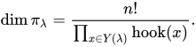
The figure on the right shows hook-lengths for all boxes in the diagram of the partition 10 = 5 + 4 + 1. Thus

Similarly, the dimension of the irreducible representation W(λ) of GLr corresponding to the partition λ of n (with at most r parts) is the number of semistandard Young tableaux of shape λ (containing only the entries from 1 to r), which is given by the hook-length formula:
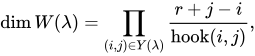
where the index i gives the row and j the column of a box.[8] For instance, for the partition (5,4,1) we get as dimension of the corresponding irreducible representation of GL7 (traversing the boxes by rows):

Restricted representations
[edit]A representation of the symmetric group on n elements, Sn is also a representation of the symmetric group on n − 1 elements, Sn−1. However, an irreducible representation of Sn may not be irreducible for Sn−1. Instead, it may be a direct sum of several representations that are irreducible for Sn−1. These representations are then called the factors of the restricted representation (see also induced representation).
The question of determining this decomposition of the restricted representation of a given irreducible representation of Sn, corresponding to a partition λ of n, is answered as follows. One forms the set of all Young diagrams that can be obtained from the diagram of shape λ by removing just one box (which must be at the end both of its row and of its column); the restricted representation then decomposes as a direct sum of the irreducible representations of Sn−1 corresponding to those diagrams, each occurring exactly once in the sum.
See also
[edit]Notes
[edit]- ^ Knuth, Donald E. (1973), The Art of Computer Programming, Vol. III: Sorting and Searching (2nd ed.), Addison-Wesley, p. 48,
Such arrangements were introduced by Alfred Young in 1900
. - ^ Young, A. (1900), "On quantitative substitutional analysis", Proceedings of the London Mathematical Society, Series 1, 33 (1): 97–145, doi:10.1112/plms/s1-33.1.97. See in particular p. 133.
- ^ Stembridge, John (1989-12-01). "On the eigenvalues of representations of reflection groups and wreath products". Pacific Journal of Mathematics. 140 (2). Mathematical Sciences Publishers: 353–396. doi:10.2140/pjm.1989.140.353. ISSN 0030-8730.
- ^ For instance the skew diagram consisting of a single square at position (2,4) can be obtained by removing the diagram of μ = (5,3,2,1) from the one of λ = (5,4,2,1), but also in (infinitely) many other ways. In general any skew diagram whose set of non-empty rows (or of non-empty columns) is not contiguous or does not contain the first row (respectively column) will be associated to more than one skew shape.
- ^ A somewhat similar situation arises for matrices: the 3-by-0 matrix A must be distinguished from the 0-by-3 matrix B, since AB is a 3-by-3 (zero) matrix while BA is the 0-by-0 matrix, but both A and B have the same (empty) set of entries; for skew tableaux however such distinction is necessary even in cases where the set of entries is not empty.
- ^ Philip R. Bunker and Per Jensen (1998) Molecular Symmetry and Spectroscopy, 2nd ed. NRC Research Press, Ottawa [1] pp.198-202.ISBN 9780660196282
- ^ R.Pauncz (1995) The Symmetric Group in Quantum Chemistry, CRC Press, Boca Raton, Florida
- ^ Predrag Cvitanović (2008). Group Theory: Birdtracks, Lie's, and Exceptional Groups. Princeton University Press., eq. 9.28 and appendix B.4
References
[edit]- William Fulton. Young Tableaux, with Applications to Representation Theory and Geometry. Cambridge University Press, 1997, ISBN 0-521-56724-6.
- Fulton, William; Harris, Joe (1991). Representation theory. A first course. Graduate Texts in Mathematics, Readings in Mathematics. Vol. 129. New York: Springer-Verlag. doi:10.1007/978-1-4612-0979-9. ISBN 978-0-387-97495-8. MR 1153249. OCLC 246650103. Lecture 4
- Howard Georgi, Lie Algebras in Particle Physics, 2nd Edition - Westview
- Macdonald, I. G. Symmetric functions and Hall polynomials. Oxford Mathematical Monographs. The Clarendon Press, Oxford University Press, Oxford, 1979. viii+180 pp. ISBN 0-19-853530-9 MR 0553598
- Laurent Manivel. Symmetric Functions, Schubert Polynomials, and Degeneracy Loci. American Mathematical Society.
- Greene, Curtis; Nijenhuis, Albert; Wilf, Herbert S. (1979). "A probabilistic proof of a formula for the number of Young tableaux of a given shape". Advances in Mathematics. 31 (1). Amsterdam: Elsevier: 104–109. doi:10.1016/0001-8708(79)90023-9. MR 0521470. Zbl 0398.05008.
- Jean-Christophe Novelli, Igor Pak, Alexander V. Stoyanovskii, "A direct bijective proof of the Hook-length formula", Discrete Mathematics and Theoretical Computer Science 1 (1997), pp. 53–67.
- Bruce E. Sagan. The Symmetric Group. Springer, 2001, ISBN 0-387-95067-2
- Vinberg, E.B. (2001) [1994], "Young tableau", Encyclopedia of Mathematics, EMS Press
- Yong, Alexander (February 2007). "What is...a Young Tableau?" (PDF). Notices of the American Mathematical Society. 54 (2): 240–241. Retrieved 2008-01-16.
- Predrag Cvitanović, Group Theory: Birdtracks, Lie's, and Exceptional Groups. Princeton University Press, 2008.
External links
[edit]- Eric W. Weisstein. "Ferrers Diagram". From MathWorld—A Wolfram Web Resource.
- Eric W. Weisstein. "Young Tableau." From MathWorld—A Wolfram Web Resource.
- Semistandard tableaux entry in the FindStat database
- Standard tableaux entry in the FindStat database
Young tableau
View on GrokipediaDefinitions and Fundamentals
Young Diagrams
A Young diagram, also known as a Ferrers diagram in its dot representation, is a left-justified array of boxes arranged in rows of nonincreasing lengths, where the lengths correspond to the parts of an integer partition λ = (λ₁ ≥ λ₂ ≥ ⋯ ≥ λ_k > 0) of a positive integer n, and the i-th row contains exactly λ_i boxes.[4][5] This geometric structure visually encodes the partition by stacking rows such that the total number of boxes equals n, with rows aligned to the left and decreasing in length from top to bottom.[6] The conjugate partition λ' of λ is obtained by transposing the Young diagram, which involves reflecting it over the main diagonal to read the lengths of the columns as the new row lengths.[7] For instance, if λ = (4, 2, 1), the diagram has four boxes in the first row, two in the second, and one in the third; its conjugate λ' = (3, 1, 1, 1) reflects the three boxes in the first column, one in the second, one in the third, and one in the fourth.[7] A partition is self-conjugate if λ = λ', such as λ = (3, 2, 1), where the diagram is symmetric across the diagonal:□ □ □
□ □
□
| (1,1) | (1,2) | (1,3) |
|---|---|---|
| 5 | 3 | 1 |
| 3 | 1 | |
| 1 |
Young Tableaux
A Young tableau is formed by filling the boxes of a Young diagram with numbers according to specific monotonicity rules, extending the geometric structure of the diagram into a combinatorial object used in various areas of mathematics.[8] A standard Young tableau (SYT) of a given shape λ, where λ is a partition of n (denoted λ ⊢ n), consists of a bijective assignment of the integers 1 through n to the n boxes of the diagram such that the entries are strictly increasing from left to right along each row and from top to bottom along each column.[1] This ensures that each SYT represents a unique way to order the numbers while respecting the partial order imposed by the diagram's rows and columns. For example, the partition λ = (2,1) has two standard Young tableaux:1 2
3
1 3
2
1 1
2
Variations
Skew tableaux generalize the concept of Young tableaux by allowing fillings on skew diagrams, which are the boxes of a Young diagram minus the boxes of a subdiagram , where and are partitions with for tableaux of size . A standard skew Young tableau of shape is a bijective filling of the skew diagram with such that entries strictly increase along each row from left to right and along each column from top to bottom.[10] Similarly, a semistandard skew Young tableau of shape fills the diagram with positive integers that are weakly increasing in rows and strictly increasing in columns, allowing repetitions but unbounded from above.[11] Reverse plane partitions extend the filling rules further by relaxing the strictness and bijectivity requirements. A reverse plane partition of shape is a filling of the Young diagram with non-negative integers that are weakly increasing along rows from left to right and along columns from top to bottom, with no upper bound on entries and repetitions permitted. This contrasts with standard plane partitions, which are weakly decreasing in both directions, but reverse versions arise naturally in generating functions and symmetric function theory. Plane partitions serve as three-dimensional analogs to Young tableaux, representing stacked layers of boxes in the positive octant that form a stable pile, equivalent to a finite subset of satisfying a stability condition where no box floats without support from below or to the side.[12] These can be visualized as a Young diagram in each horizontal slice, with heights constrained by the partition shape, effectively generalizing two-dimensional tableaux to a boxed, multi-layered structure. For example, consider the skew shape , which consists of four boxes: positions , , , and . One standard skew Young tableau filling is: 1 2
3 4
  2  4
1  3
Combinatorial Properties
Hook-Length Formula
The hook-length formula provides an explicit product formula for the number of standard Young tableaux of a given shape , where is a partition of the integer . For a cell in the Young diagram of , the hook length is the number of cells to the right of in row , plus the number of cells below in column , plus one for the cell itself. The formula states that| 1 | (1) | 1 |
| 2 | (2) | 1 |
| (1,1) | 1 | |
| 3 | (3) | 1 |
| (2,1) | 2 | |
| (1^3) | 1 | |
| 4 | (4) | 1 |
| (3,1) | 3 | |
| (2,2) | 2 | |
| (2,1,1) | 3 | |
| (1^4) | 1 | |
| 5 | (5) | 1 |
| (4,1) | 4 | |
| (3,2) | 5 | |
| (3,1,1) | 6 | |
| (2,2,1) | 5 | |
| (2,1^3) | 6 | |
| (1^5) | 1 |
RSK Correspondence
The Robinson–Schensted–Knuth (RSK) correspondence is a fundamental bijection in combinatorics that associates permutations in the symmetric group with pairs of standard Young tableaux of the same shape, where is the insertion tableau and is the recording tableau.[16] This correspondence was first introduced by G. de B. Robinson in 1938 as a method to decompose the regular representation of the symmetric group using tableaux, though without a full bijective proof.[16] It was rediscovered and rigorously established as a bijection by C. Schensted in 1961, who connected it to the lengths of longest increasing and decreasing subsequences in permutations. In 1970, D. E. Knuth generalized the algorithm to non-negative integer matrices, yielding a bijection with pairs of semistandard Young tableaux (SSYT) of the same shape, and introduced relations characterizing equivalence classes of inputs that produce the same output shape. Central to the RSK correspondence is Schensted insertion, an algorithm for building the insertion tableau while maintaining the increasing properties of rows and columns. To insert a number into an existing Young tableau, begin with the first row: place in the leftmost position where it is smaller than the entry to its right, displacing (or "bumping") that entry to the next row; if no such position exists, append to the end of the row. The bumped entry then repeats the process in the subsequent row, continuing until an entry is appended to the end of some row, which adds a new box to the shape. This ensures the resulting tableau remains row- and column-strictly increasing. For a permutation viewed as the sequence , the insertion tableau is obtained by successively inserting these values using Schensted insertion, starting from an empty tableau; simultaneously, the recording tableau is built by placing the index (from 1 to ) in the new box added at the -th step, ensuring both and are standard Young tableaux of the same shape . The map is bijective, with the inverse recovered via reverse bumping or jeu de taquin procedures. For example, consider the permutation 231, given by the sequence 2, 3, 1. Inserting 2 yields . Inserting 3 appends to the first row, giving . Inserting 1 into (2, 3) bumps 2 (the leftmost entry >1), resulting in first row (1, 3) and second row (2), so . The recording tableau records the steps: 1 at the first box, 2 at the second box in the first row, and 3 at the new box in the second row, yielding . The inverse process recovers the original sequence 2, 3, 1 from . Knuth's 1970 extension generalizes the correspondence to matrices with non-negative integer entries, associating each such matrix with a pair of SSYT of the same shape, where entries in rows are weakly increasing and in columns strictly increasing. The algorithm processes the matrix column by column (or row by row in variants), inserting each entry via a generalized Schensted insertion that allows equal entries without bumping. Two-line arrays (with top row strictly increasing and bottom row arbitrary non-negative integers) map to such pairs, and the shape is preserved under Knuth equivalence classes: two arrays are equivalent if one can be obtained from the other by a sequence of Knuth relations, such as swapping adjacent entries with or similar transpositions that do not change the resulting tableaux pair. These relations define the plactic monoid structure underlying the correspondence.Applications in Algebra and Representation Theory
Schur Polynomials
Schur polynomials provide a fundamental connection between the combinatorics of Young tableaux and the algebra of symmetric functions. For a partition and variables , the Schur polynomial is defined as the sum over all semistandard Young tableaux of shape with entries from , of the monomial , where denotes the multiplicity of in .[17] This combinatorial definition leverages semistandard Young tableaux, which feature weakly increasing rows and strictly increasing columns, to generate a homogeneous symmetric polynomial of degree .[17] Key properties of Schur polynomials highlight their role in representation theory. They serve as the characters of the irreducible representations of the symmetric group indexed by , where the character value on a conjugacy class corresponding to partition is obtained by evaluating the Schur polynomial appropriately.[17] Additionally, Schur polynomials form an orthonormal basis for the ring of symmetric functions with respect to the Hall inner product, ensuring .[18] The Pieri rule provides a basic multiplication formula: , where the sum is over partitions such that is a horizontal strip of boxes.[19] The Jacobi-Trudi identity offers an alternative generating function expression for Schur polynomials in terms of complete homogeneous symmetric polynomials . Specifically,Representations of Symmetric Groups
The irreducible representations of the symmetric group over the complex numbers are in one-to-one correspondence with the partitions , where each partition labels a unique irreducible representation known as the Specht module .1 These modules provide a combinatorial framework for understanding the representation theory of , with Young tableaux serving as the key tool for constructing bases and computing invariants. The Specht modules were first constructed by Wilhelm Specht in 1935, building on earlier work by Alfred Young that linked tableaux to group representations.2 The Specht module is defined as a submodule of the permutation module , which has basis given by the tabloids formed by equivalence classes of Young tableaux of shape under row permutations.1 Specifically, is spanned by the polytabloids , where is the column stabilizer group of the tableau , and a standard basis consists of polytabloids for standard Young tableaux (SYT) of shape .3 The group acts on by permuting the entries in the tableaux, with , preserving the submodule structure.1 These modules are irreducible, and they exhaust all irreducible representations of , providing a complete classification parameterized by Young diagrams.3 The dimension of is given by , the number of standard Young tableaux of shape .1 This quantity can be computed using the hook-length formula, which counts SYT via products over hook lengths in the diagram.4 The dimensions satisfy the orthogonality relation , reflecting the decomposition of the regular representation of .1 The character of the representation evaluates on a permutation as , which counts certain fixed points or can be computed combinatorially.1 One method uses the Robinson-Schensted-Knuth (RSK) correspondence, where relates to the number of pairs of tableaux of shape arising from the insertion and recording of .5 Alternatively, the Murnaghan-Nakayama rule provides a recursive formula: , summing over rim hooks of length equal to a part of the cycle type of , where is the height of the hook.67 For , the partitions are , , and , corresponding to the trivial representation (), the standard representation (), and the sign representation (), respectively.1 The two SYT of shape are:1 2
3
1 3
2