
Recent from talks
Crank–Nicolson method
Knowledge base stats:
Talk channels stats:
Members stats:
Crank–Nicolson method
In numerical analysis, the Crank–Nicolson method is a finite difference method used for numerically solving the heat equation and similar partial differential equations. It is a second-order method in time. It is implicit in time, can be written as an implicit Runge–Kutta method, and it is numerically stable. The method was developed by John Crank and Phyllis Nicolson in the 1940s.
For diffusion equations (and many other equations), it can be shown the Crank–Nicolson method is unconditionally stable. However, the approximate solutions can still contain (decaying) spurious oscillations if the ratio of time step times the thermal diffusivity to the square of space step, , is large (typically, larger than 1/2 per Von Neumann stability analysis). For this reason, whenever large time steps or high spatial resolution is necessary, the less accurate backward Euler method is often used, which is both stable and immune to oscillations.[citation needed]


The Crank–Nicolson method is based on the trapezoidal rule, giving second-order convergence in time. For linear equations, the trapezoidal rule is equivalent to the implicit midpoint method[citation needed]—the simplest example of a Gauss–Legendre implicit Runge–Kutta method—which also has the property of being a geometric integrator. For example, in one dimension, suppose the partial differential equation is
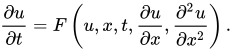
Letting and evaluated for and , the equation for Crank–Nicolson method is a combination of the forward Euler method at and the backward Euler method at (note, however, that the method itself is not simply the average of those two methods, as the backward Euler equation has an implicit dependence on the solution):



Note that this is an implicit method: to get the "next" value of in time, a system of algebraic equations must be solved. If the partial differential equation is nonlinear, the discretization will also be nonlinear, so that advancing in time will involve the solution of a system of nonlinear algebraic equations, though linearizations are possible. In many problems, especially linear diffusion, the algebraic problem is tridiagonal and may be efficiently solved with the tridiagonal matrix algorithm, which gives a fast direct solution, as opposed to the usual for a full matrix, in which indicates the matrix size.


The Crank–Nicolson method is often applied to diffusion problems. As an example, for linear diffusion,
applying a finite difference spatial discretization for the right-hand side, the Crank–Nicolson discretization is then
or, letting ,

Hub AI
Crank–Nicolson method AI simulator
(@Crank–Nicolson method_simulator)
Crank–Nicolson method
In numerical analysis, the Crank–Nicolson method is a finite difference method used for numerically solving the heat equation and similar partial differential equations. It is a second-order method in time. It is implicit in time, can be written as an implicit Runge–Kutta method, and it is numerically stable. The method was developed by John Crank and Phyllis Nicolson in the 1940s.
For diffusion equations (and many other equations), it can be shown the Crank–Nicolson method is unconditionally stable. However, the approximate solutions can still contain (decaying) spurious oscillations if the ratio of time step times the thermal diffusivity to the square of space step, , is large (typically, larger than 1/2 per Von Neumann stability analysis). For this reason, whenever large time steps or high spatial resolution is necessary, the less accurate backward Euler method is often used, which is both stable and immune to oscillations.[citation needed]
The Crank–Nicolson method is based on the trapezoidal rule, giving second-order convergence in time. For linear equations, the trapezoidal rule is equivalent to the implicit midpoint method[citation needed]—the simplest example of a Gauss–Legendre implicit Runge–Kutta method—which also has the property of being a geometric integrator. For example, in one dimension, suppose the partial differential equation is
Letting and evaluated for and , the equation for Crank–Nicolson method is a combination of the forward Euler method at and the backward Euler method at (note, however, that the method itself is not simply the average of those two methods, as the backward Euler equation has an implicit dependence on the solution):
Note that this is an implicit method: to get the "next" value of in time, a system of algebraic equations must be solved. If the partial differential equation is nonlinear, the discretization will also be nonlinear, so that advancing in time will involve the solution of a system of nonlinear algebraic equations, though linearizations are possible. In many problems, especially linear diffusion, the algebraic problem is tridiagonal and may be efficiently solved with the tridiagonal matrix algorithm, which gives a fast direct solution, as opposed to the usual for a full matrix, in which indicates the matrix size.
The Crank–Nicolson method is often applied to diffusion problems. As an example, for linear diffusion,
applying a finite difference spatial discretization for the right-hand side, the Crank–Nicolson discretization is then
or, letting ,