In the calculus of variations and classical mechanics, the Euler–Lagrange equations are a system of second-order ordinary differential equations whose solutions are stationary points of the given action functional. The equations were discovered in the 1750s by Swiss mathematician Leonhard Euler and Italian mathematician Joseph-Louis Lagrange.

Because a differentiable functional is stationary at its local extrema, the Euler–Lagrange equation is useful for solving optimization problems in which, given some functional, one seeks the function minimizing or maximizing it. This is analogous to Fermat's theorem in calculus, stating that at any point where a differentiable function attains a local extremum its derivative is zero. In Lagrangian mechanics, according to Hamilton's principle of stationary action, the evolution of a physical system is described by the solutions to the Euler equation for the action of the system. In this context Euler equations are usually called Lagrange equations. In classical mechanics, it is equivalent to Newton's laws of motion; indeed, the Euler-Lagrange equations will produce the same equations as Newton's Laws. This is particularly useful when analyzing systems whose force vectors are particularly complicated. It has the advantage that it takes the same form in any system of generalized coordinates, and it is better suited to generalizations. In classical field theory there is an analogous equation to calculate the dynamics of a field.

The Euler–Lagrange equation was developed in the 1750s by Euler and Lagrange in connection with their studies of the tautochrone problem. This is the problem of determining a curve on which a weighted particle will fall to a fixed point in a fixed amount of time, independent of the starting point.

Lagrange solved this problem in 1755 and sent the solution to Euler. Both further developed Lagrange's method and applied it to mechanics, which led to the formulation of Lagrangian mechanics. Their correspondence ultimately led to the calculus of variations, a term coined by Euler himself in 1766.

Let ${\displaystyle (X,L)}$ be a real dynamical system with ${\displaystyle n}$ degrees of freedom. Here ${\displaystyle X}$ is the configuration space and ${\displaystyle L=L(t,{\boldsymbol {q}}(t),{\boldsymbol {v}}(t))}$ the Lagrangian, i.e. a smooth real-valued function such that ${\displaystyle {\boldsymbol {q}}(t)\in X,}$ and ${\displaystyle {\boldsymbol {v}}(t)}$ is an ${\displaystyle n}$-dimensional "vector of speed". (For those familiar with differential geometry, ${\displaystyle X}$ is a smooth manifold, and ${\displaystyle L\colon {\mathbb {R} }_{t}\times TX\to {\mathbb {R} },}$ where ${\displaystyle TX}$ is the tangent bundle of ${\displaystyle X).}$

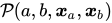
Let ${\displaystyle {\cal {P}}(a,b,{\boldsymbol {x}}_{a},{\boldsymbol {x}}_{b})}$ be the set of smooth paths ${\displaystyle {\boldsymbol {q}}:[a,b]\to X}$ for which ${\displaystyle {\boldsymbol {q}}(a)={\boldsymbol {x}}_{a}}$ and ${\displaystyle {\boldsymbol {q}}(b)={\boldsymbol {x}}_{b}.}$

The action functional ${\displaystyle S\colon {\cal {P}}(a,b,{\boldsymbol {x}}_{a},{\boldsymbol {x}}_{b})\to \mathbb {R} }$ is defined via $${\displaystyle S[{\boldsymbol {q}}]=\int _{a}^{b}L(t,{\boldsymbol {q}}(t),{\dot {\boldsymbol {q}}}(t))\,dt.}$$

A path ${\displaystyle {\boldsymbol {q}}\in {\cal {P}}(a,b,{\boldsymbol {x}}_{a},{\boldsymbol {x}}_{b})}$ is a stationary point of ${\displaystyle S}$ if and only if