Characteristic polynomial
Main page

Characteristic polynomial

logo
Community Hub0 subscribers
Read side by side
from Wikipedia

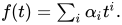
In linear algebra, the characteristic polynomial of a square matrix is a polynomial which is invariant under matrix similarity and has the eigenvalues as roots. It has the determinant and the trace of the matrix among its coefficients. The characteristic polynomial of an endomorphism of a finite-dimensional vector space is the characteristic polynomial of the matrix of that endomorphism over any basis (that is, the characteristic polynomial does not depend on the choice of a basis). The characteristic equation, also known as the determinantal equation,[1][2][3] is the equation obtained by equating the characteristic polynomial to zero.

In spectral graph theory, the characteristic polynomial of a graph is the characteristic polynomial of its adjacency matrix.[4]

Motivation

[edit]

In linear algebra, eigenvalues and eigenvectors play a fundamental role, since, given a linear transformation, an eigenvector is a vector whose direction is not changed by the transformation, and the corresponding eigenvalue is the measure of the resulting change of magnitude of the vector.

More precisely, suppose the transformation is represented by a square matrix Then an eigenvector and the corresponding eigenvalue must satisfy the equation or, equivalently (since ), where is the identity matrix, and (although the zero vector satisfies this equation for every it is not considered an eigenvector).

It follows that the matrix must be singular, and its determinant must be zero.

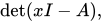
In other words, the eigenvalues of A are the roots of which is a monic polynomial in x of degree n if A is a n×n matrix. This polynomial is the characteristic polynomial of A.
Formal definition

[edit]

Consider an matrix The characteristic polynomial of denoted by is the polynomial defined by[5] where denotes the identity matrix.

Some authors define the characteristic polynomial to be That polynomial differs from the one defined here by a sign so it makes no difference for properties like having as roots the eigenvalues of ; however the definition above always gives a monic polynomial, whereas the alternative definition is monic only when is even.

Examples

[edit]

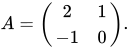
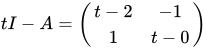
To compute the characteristic polynomial of the matrix the determinant of the following is computed: and found to be the characteristic polynomial of
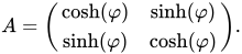
Another example uses hyperbolic functions of a hyperbolic angle φ. For the matrix take Its characteristic polynomial is

Properties

[edit]

The characteristic polynomial of a matrix is monic (its leading coefficient is ) and its degree is The most important fact about the characteristic polynomial was already mentioned in the motivational paragraph: the eigenvalues of are precisely the roots of (this also holds for the minimal polynomial of but its degree may be less than ). All coefficients of the characteristic polynomial are polynomial expressions in the entries of the matrix. In particular its constant coefficient of is the coefficient of is 1, and the coefficient of is tr(−A) = −tr(A), where tr(A) is the trace of (The signs given here correspond to the formal definition given in the previous section; for the alternative definition these would instead be and (−1)n – 1 tr(A) respectively.[6])

For a matrix the characteristic polynomial is thus given by

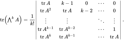
Using the language of exterior algebra, the characteristic polynomial of an matrix may be expressed as where is the trace of the th exterior power of which has dimension This trace may be computed as the sum of all principal minors of of size The recursive Faddeev–LeVerrier algorithm computes these coefficients more efficiently [clarification needed].
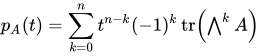
When the characteristic of the field of the coefficients is each such trace may alternatively be computed as a single determinant, that of the matrix,

The Cayley–Hamilton theorem states that replacing by in the characteristic polynomial (interpreting the resulting powers as matrix powers, and the constant term as times the identity matrix) yields the zero matrix. Informally speaking, every matrix satisfies its own characteristic equation. This statement is equivalent to saying that the minimal polynomial of divides the characteristic polynomial of

Two similar matrices have the same characteristic polynomial. The converse however is not true in general: two matrices with the same characteristic polynomial need not be similar.

The matrix and its transpose have the same characteristic polynomial. is similar to a triangular matrix if and only if its characteristic polynomial can be completely factored into linear factors over (the same is true with the minimal polynomial instead of the characteristic polynomial). In this case is similar to a matrix in Jordan normal form.

Characteristic polynomial of a product of two matrices

[edit]

If and are two square matrices then characteristic polynomials of and coincide:

Proof: If is a non-zero generalized eigenvalue of of algebraic multiplicity , and belongs to the kernel of , then belongs to the kernel of , so the non-zero generalized eigenspaces of and have the same dimension. Therefore, since and are both , the remaining generalized eigenspaces, with eigenvalue 0, have the same dimension. Therefore and have the same characteristic polynomial, because all generalized eigenvalues are the same, with the same algebraic multiplicities.

More generally, if is a matrix of order and is a matrix of order then is and is matrix, and one has

To prove this, one may suppose by exchanging, if needed, and Then, by bordering on the bottom by rows of zeros, and on the right, by, columns of zeros, one gets two matrices and such that and is equal to bordered by rows and columns of zeros. The result follows from the case of square matrices, by comparing the characteristic polynomials of and

Characteristic polynomial of Ak

[edit]

If is an eigenvalue of a square matrix with eigenvector then is an eigenvalue of because

The multiplicities can be shown to agree as well, and this generalizes to any polynomial in place of :[7]

Theorem Let be a square matrix and let be a polynomial. If the characteristic polynomial of has a factorization then the characteristic polynomial of the matrix is given by

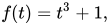
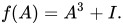
That is, the algebraic multiplicity of in equals the sum of algebraic multiplicities of in over such that In particular, and Here a polynomial for example, is evaluated on a matrix simply as

The theorem applies to matrices and polynomials over any field or commutative ring.[8] However, the assumption that has a factorization into linear factors is not always true, unless the matrix is over an algebraically closed field such as the complex numbers.

Proof

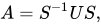
This proof only applies to matrices and polynomials over complex numbers (or any algebraically closed field). In that case, the characteristic polynomial of any square matrix can be always factorized as where are the eigenvalues of possibly repeated. Moreover, the Jordan decomposition theorem guarantees that any square matrix can be decomposed as where is an invertible matrix and is upper triangular with on the diagonal (with each eigenvalue repeated according to its algebraic multiplicity). (The Jordan normal form has stronger properties, but these are sufficient; alternatively the Schur decomposition can be used, which is less popular but somewhat easier to prove).

Let Then For an upper triangular matrix with diagonal the matrix is upper triangular with diagonal in and hence is upper triangular with diagonal Therefore, the eigenvalues of are Since is similar to it has the same eigenvalues, with the same algebraic multiplicities.


Secular function and secular equation

[edit]

Secular function

[edit]

The term secular function has been used for what is now called characteristic polynomial (in some literature the term secular function is still used). The term comes from the fact that the characteristic polynomial was used to calculate secular perturbations (on a time scale of a century, that is, slow compared to annual motion) of planetary orbits, according to Lagrange's theory of oscillations.

Secular equation

[edit]

Secular equation may have several meanings.

  • In linear algebra it is sometimes used in place of characteristic equation.
  • In astronomy it is the algebraic or numerical expression of the magnitude of the inequalities in a planet's motion that remain after the inequalities of a short period have been allowed for.[9]
  • In molecular orbital calculations relating to the energy of the electron and its wave function it is also used instead of the characteristic equation.

For general associative algebras

[edit]

The above definition of the characteristic polynomial of a matrix with entries in a field generalizes without any changes to the case when is just a commutative ring. Garibaldi (2004) defines the characteristic polynomial for elements of an arbitrary finite-dimensional (associative, but not necessarily commutative) algebra over a field and proves the standard properties of the characteristic polynomial in this generality.

See also

[edit]

References

[edit]
Revisions and contributorsEdit on WikipediaRead on Wikipedia
from Grokipedia
In linear algebra, the characteristic polynomial of an $ n \times n $ square matrix $ A $ is defined as $ p_A(\lambda) = \det(\lambda I - A) $, where $ I $ is the $ n \times n $ identity matrix and $ \lambda $ is a scalar variable; this yields a monic polynomial of degree $ n $ whose roots are the eigenvalues of $ A $.[1][2] The characteristic polynomial is invariant under similarity transformations, meaning that if $ B = P^{-1} A P $ for some invertible matrix $ P $, then $ p_B(\lambda) = p_A(\lambda) $, which underscores its role in capturing intrinsic spectral properties of the matrix independent of basis choice.[2] The coefficients of the polynomial are related to the traces of powers of $ A $ via Newton identities, providing connections to other matrix invariants like the determinant (the constant term, up to sign) and the trace (the coefficient of $ \lambda^{n-1} $, up to sign).[3] A cornerstone result involving the characteristic polynomial is the Cayley–Hamilton theorem, which states that every square matrix satisfies its own characteristic equation, so $ p_A(A) = 0 $; this theorem, first appearing in Arthur Cayley's 1858 work on matrices, enables efficient computation of high powers of matrices and has broad implications in algebra and analysis.[2][4] The characteristic polynomial plays a pivotal role in spectral theory, facilitating the computation of eigenvalues and eigenvectors essential for diagonalization and Jordan canonical form, and extends to applications in control theory for system stability analysis, quantum mechanics for operator spectra, and numerical methods for solving differential equations.[1][5]

Basic Concepts

Motivation

The concept of the characteristic polynomial emerges from the fundamental quest in linear algebra to identify the eigenvalues of a matrix, which reveal essential properties of the associated linear transformation. Consider a square matrix AA representing a linear operator on a vector space. An eigenvalue λ\lambda is a scalar for which there exists a non-zero vector vv (an eigenvector) satisfying Av=λvA v = \lambda v. Rearranging this equation yields (AλI)v=0(A - \lambda I) v = 0, where II is the identity matrix. For this homogeneous system to have a non-trivial solution, the matrix AλIA - \lambda I must be singular, meaning its determinant vanishes: det(AλI)=0\det(A - \lambda I) = 0. To obtain a monic polynomial (leading coefficient 1), the characteristic polynomial is conventionally defined using det(λIA)\det(\lambda I - A), whose roots are precisely the eigenvalues of AA. This connection provides a polynomial equation whose solutions characterize the scaling factors of the transformation along certain directions.[6] This polynomial arises naturally from expanding the determinant det(λIA)\det(\lambda I - A), which for an n×nn \times n matrix AA produces a degree-nn polynomial in λ\lambda. The brief derivation begins with the matrix λIA\lambda I - A, whose entries are linear in λ\lambda; the determinant, being a multilinear function of the rows (or columns), expands into a sum of terms, each contributing powers of λ\lambda up to nn, with the constant term being (1)ndet(A)(-1)^n \det(A). This structure encodes the condition for the kernel of λIA\lambda I - A to be non-trivial, directly linking the polynomial's roots to the spectrum of AA.[6] Historically, the characteristic polynomial was developed by Augustin-Louis Cauchy in his 1829 memoir "Sur l'équation à l'aide de laquelle on détermine les inégalités séculaires des mouvements des planètes," where he employed it in the context of celestial mechanics to analyze secular perturbations in planetary orbits, using linear substitutions and quadratic forms. In this work, Cauchy introduced the term "characteristic equation" (équation caractéristique) and "characteristic root" (racine caractéristique), and demonstrated that the eigenvalues of symmetric matrices are real, marking a pivotal advancement in the spectral theory of matrices. This laid the groundwork for later developments in operator theory and quantum mechanics, where spectral properties underpin the decomposition of transformations.[7] Intuitively, the "characteristic" nature of the polynomial stems from its invariance under similarity transformations: if B=P1APB = P^{-1} A P for an invertible matrix PP, then det(λIB)=det(λIP1AP)=det(P1(λIA)P)=det(λIA)\det(\lambda I - B) = \det(\lambda I - P^{-1} A P) = \det(P^{-1} (\lambda I - A) P) = \det(\lambda I - A), preserving the polynomial. This invariance ensures that the characteristic polynomial captures intrinsic behavioral traits of the linear transformation, independent of the basis chosen to represent the matrix, making it a robust descriptor of the operator's spectrum.[8]

Formal Definition

The characteristic polynomial of an n×nn \times n matrix AA with entries in a field FF is defined as the polynomial pA(λ)=det(λInA)p_A(\lambda) = \det(\lambda I_n - A) in the polynomial ring F[λ]F[\lambda], where InI_n denotes the n×nn \times n identity matrix and det\det is the determinant function over FF.[8][9] This polynomial has degree nn and is monic, meaning its leading coefficient is 1, because the leading term arises from det(λIn)=λn\det(\lambda I_n) = \lambda^n, with lower-degree terms contributed by the entries of A-A.[8] Common notations for the characteristic polynomial include pA(λ)p_A(\lambda) or χA(λ)\chi_A(\lambda). Some texts define it as det(AλIn)\det(A - \lambda I_n), which equals (1)ndet(λInA)(-1)^n \det(\lambda I_n - A), introducing a sign alternation depending on the parity of nn; in such cases, the monic version is obtained by multiplying by (1)n(-1)^n to ensure the leading coefficient is 1.[3][10] More generally, for an endomorphism TT (a linear map from a finite-dimensional vector space VV over FF to itself), the characteristic polynomial pT(λ)p_T(\lambda) is defined using any matrix representation AA of TT with respect to a basis of VV, yielding pT(λ)=det(λIA)p_T(\lambda) = \det(\lambda I - A); this is independent of the choice of basis, as similar matrices share the same characteristic polynomial.[9]

Illustrative Examples

Low-Dimensional Matrices

For the simplest case of a 1×11 \times 1 matrix A=[a]A = [a], the characteristic polynomial is computed as p(λ)=λap(\lambda) = \lambda - a.[3][11] This linear polynomial directly reflects the matrix's single entry, and its root λ=a\lambda = a is the eigenvalue of AA.[3][11] Consider a general 2×22 \times 2 matrix A=(abcd)A = \begin{pmatrix} a & b \\ c & d \end{pmatrix}. The characteristic polynomial is p(λ)=det(λIA)p(\lambda) = \det(\lambda I - A), which expands to the determinant of (λabcλd)\begin{pmatrix} \lambda - a & -b \\ -c & \lambda - d \end{pmatrix}. Expanding this determinant gives (λa)(λd)(b)(c)=λ2(a+d)λ+(adbc)(\lambda - a)(\lambda - d) - (-b)(-c) = \lambda^2 - (a + d)\lambda + (ad - bc).[3][11] The roots of this quadratic polynomial are the eigenvalues of AA, accounting for any multiplicity if repeated.[3][11] For a 3×33 \times 3 diagonal matrix A=diag(λ1,λ2,λ3)A = \operatorname{diag}(\lambda_1, \lambda_2, \lambda_3), the characteristic polynomial simplifies to p(λ)=(λλ1)(λλ2)(λλ3)p(\lambda) = (\lambda - \lambda_1)(\lambda - \lambda_2)(\lambda - \lambda_3).[3][11] This product form arises because the off-diagonal entries are zero, making the determinant a straightforward multiplication of the diagonal terms after subtracting λI\lambda I. The roots λ1,λ2,λ3\lambda_1, \lambda_2, \lambda_3 are precisely the eigenvalues, each with algebraic multiplicity one unless values repeat.[3][11] In all these low-dimensional cases, the roots of the characteristic polynomial correspond to the eigenvalues of the matrix, with multiplicities indicating how many times each eigenvalue appears.[3][11] This connection holds generally, as the eigenvalues solve det(λIA)=0\det(\lambda I - A) = 0.[3]

Structured Matrices

Matrices with specific structures often admit simplified expressions for their characteristic polynomials, revealing direct connections between the matrix entries and the eigenvalues. For a diagonal matrix $ D = \operatorname{diag}(d_1, d_2, \dots, d_n) $, the characteristic polynomial is given by $ \det(\lambda I - D) = \prod_{i=1}^n (\lambda - d_i) $. In this case, the eigenvalues are precisely the diagonal entries $ d_i $, and the polynomial factors completely into linear terms corresponding to these values.[11] Upper and lower triangular matrices exhibit a similar property. For an upper triangular matrix $ T $ with diagonal entries $ t_1, t_2, \dots, t_n $, the characteristic polynomial is $ \det(\lambda I - T) = \prod_{i=1}^n (\lambda - t_i) $, as the determinant of $ \lambda I - T $ is the product of the diagonal entries due to its triangular form. The eigenvalues are thus the diagonal elements, independent of the entries above (or below, for lower triangular) the diagonal. This holds analogously for lower triangular matrices.[12] The companion matrix provides a canonical construction linking a monic polynomial directly to a matrix whose characteristic polynomial matches it. For a monic polynomial $ p(\lambda) = \lambda^n + a_{n-1} \lambda^{n-1} + \cdots + a_1 \lambda + a_0 $, the companion matrix $ C $ is the $ n \times n $ matrix with subdiagonal entries of 1 (i.e., 1's on the first subdiagonal and zeros elsewhere below), the last column consisting of $ -a_0, -a_1, \dots, -a_{n-1} $ in the rows from bottom to top, and zeros above the subdiagonal in the first $ n-1 $ columns. Explicitly,
C=(000a0100a1010a2001an1). C = \begin{pmatrix} 0 & 0 & \cdots & 0 & -a_0 \\ 1 & 0 & \cdots & 0 & -a_1 \\ 0 & 1 & \cdots & 0 & -a_2 \\ \vdots & \vdots & \ddots & \vdots & \vdots \\ 0 & 0 & \cdots & 1 & -a_{n-1} \end{pmatrix}.
The characteristic polynomial of $ C $ is exactly $ p(\lambda) $, as $ \det(\lambda I - C) = p(\lambda) $, which follows from expanding the determinant along the first row and using induction on the polynomial degree. This construction is fundamental for realizing any monic polynomial as the characteristic polynomial of some matrix.[13] A Jordan block $ J_k(\mu) $ of size $ k $ with eigenvalue $ \mu $ is an upper triangular matrix with $ \mu $ on the diagonal and 1's on the superdiagonal, zeros elsewhere:
Jk(μ)=(μ1000μ1000μ1000μ). J_k(\mu) = \begin{pmatrix} \mu & 1 & 0 & \cdots & 0 \\ 0 & \mu & 1 & \cdots & 0 \\ \vdots & \vdots & \ddots & \ddots & \vdots \\ 0 & 0 & \cdots & \mu & 1 \\ 0 & 0 & \cdots & 0 & \mu \end{pmatrix}.
Its characteristic polynomial is $ (\lambda - \mu)^k $, reflecting the algebraic multiplicity $ k $ of the eigenvalue $ \mu $, with all eigenvalues equal to $ \mu $. This arises because $ \lambda I - J_k(\mu) $ is upper triangular with $ \lambda - \mu $ on the diagonal.

Algebraic Properties

Invariance and Trace Relations

One fundamental property of the characteristic polynomial $ p_A(\lambda) = \det(\lambda I - A) $ of an $ n \times n $ matrix $ A $ is its invariance under similarity transformations. Specifically, if $ P $ is an invertible matrix, then the characteristic polynomial of $ P^{-1} A P $ equals that of $ A $: $ p_{P^{-1} A P}(\lambda) = p_A(\lambda) $. This follows from the determinant identity
det(λIP1AP)=det(P1(λIA)P)=det(P1)det(λIA)det(P)=det(λIA), \det(\lambda I - P^{-1} A P) = \det(P^{-1} (\lambda I - A) P) = \det(P^{-1}) \det(\lambda I - A) \det(P) = \det(\lambda I - A),
since $ \det(P^{-1}) \det(P) = 1 $.[11] This invariance underscores the characteristic polynomial's role as a similarity invariant, capturing essential spectral information independent of the basis chosen for the matrix representation.[14] The coefficients of the characteristic polynomial connect directly to key matrix invariants through Vieta's formulas, applied to its roots—the eigenvalues of $ A $ counted with algebraic multiplicity. For the monic polynomial $ p_A(\lambda) = \lambda^n + c_{n-1} \lambda^{n-1} + \cdots + c_1 \lambda + c_0 $, the sum of the roots (with sign) is $ -c_{n-1} $, so the trace of $ A $, $ \operatorname{tr}(A) $, equals the negative of the coefficient of $ \lambda^{n-1} $, or $ \operatorname{tr}(A) = -\sum \lambda_i $. Similarly, the product of the roots (with sign) relates to the constant term $ c_0 = (-1)^n \prod \lambda_i $, yielding $ \det(A) = \prod \lambda_i $, up to the sign from $ \det(-A) $.[15] The leading coefficient is always 1, ensuring the polynomial is monic, while the constant term is precisely $ (-1)^n \det(A) $.[3] As the unique monic polynomial of degree $ n $ whose roots are exactly the eigenvalues of $ A $ with their algebraic multiplicities, the characteristic polynomial provides a complete algebraic encapsulation of the spectrum. This uniqueness stems from the fundamental theorem of algebra, guaranteeing that the eigenvalues are the roots with the specified multiplicities in the complex numbers, and the monic normalization distinguishes it from scalar multiples.[3]

Cayley-Hamilton Theorem

The Cayley-Hamilton theorem states that if $ A $ is an $ n \times n $ matrix over a commutative ring, and $ p_A(\lambda) = \det(\lambda I - A) = \lambda^n + c_{n-1} \lambda^{n-1} + \cdots + c_1 \lambda + c_0 $ is its characteristic polynomial, then $ p_A(A) = A^n + c_{n-1} A^{n-1} + \cdots + c_1 A + c_0 I = 0 $, the zero matrix.[16] The theorem was independently discovered by William Rowan Hamilton in 1853, who proved it in the context of inverses of linear functions of quaternions, and by Arthur Cayley in 1858, who provided a general proof for matrices in his seminal paper on matrix theory.[17][18] A standard proof uses the adjugate matrix. Recall that for any square matrix $ B $, $ B \cdot \adj(B) = \det(B) I $. Consider the characteristic matrix $ \lambda I - A $, whose adjugate is a matrix of polynomials in $ \lambda $ of degree at most $ n-1 $, say $ \adj(\lambda I - A) = \sum_{k=0}^{n-1} P_k \lambda^k $, where each $ P_k $ is an $ n \times n $ matrix with entries that are polynomials in the entries of $ A $. Then,
(λIA)\adj(λIA)=pA(λ)I. (\lambda I - A) \cdot \adj(\lambda I - A) = p_A(\lambda) I.
This is a matrix polynomial identity in $ \lambda $. Since the entries of $ A $ commute with the scalar $ \lambda $, we can formally substitute $ \lambda = A $, yielding
(AIA)\adj(AIA)=pA(A)I, (A I - A) \cdot \adj(A I - A) = p_A(A) I,
or $ 0 \cdot \adj(0) = p_A(A) I $, so $ p_A(A) = 0 $.[16][19] The theorem implies that every square matrix satisfies a monic polynomial equation of degree at most $ n $, and the minimal polynomial of the matrix, which is the monic polynomial of least degree annihilating the matrix, divides the characteristic polynomial.[8]

Special Cases

Products of Matrices

When two square matrices AA and BB of the same size commute, meaning AB=BAAB = BA, they can be simultaneously upper triangularized over the complex numbers. In this common triangular basis, the diagonal entries of the triangular form of ABAB are the products of the corresponding diagonal entries of the triangular forms of AA and BB. Consequently, the eigenvalues of ABAB (counting algebraic multiplicities) are precisely the products of the eigenvalues of AA and the eigenvalues of BB. Thus, the roots of the characteristic polynomial pAB(λ)p_{AB}(\lambda) are the products of the roots of pA(λ)p_A(\lambda) and pB(λ)p_B(\lambda), determining pAB(λ)p_{AB}(\lambda) up to the specific pairing of eigenvalues induced by the simultaneous triangularization. This multiplicative property of eigenvalues holds only under the commutativity assumption. Without commutativity, the eigenvalues of ABAB generally do not form the set of products of individual eigenvalues from AA and BB. For instance, consider the non-commuting 2×22 \times 2 matrices
A=(1101),B=(1011), A = \begin{pmatrix} 1 & 1 \\ 0 & 1 \end{pmatrix}, \quad B = \begin{pmatrix} 1 & 0 \\ 1 & 1 \end{pmatrix},
each with characteristic polynomial pA(λ)=pB(λ)=(λ1)2p_A(\lambda) = p_B(\lambda) = (\lambda - 1)^2 and eigenvalues 1,11, 1. Their product is
AB=(2111), AB = \begin{pmatrix} 2 & 1 \\ 1 & 1 \end{pmatrix},
with characteristic polynomial pAB(λ)=λ23λ+1p_{AB}(\lambda) = \lambda^2 - 3\lambda + 1 and eigenvalues 3±52\frac{3 \pm \sqrt{5}}{2}, which are not products of the eigenvalues of AA and BB. For rectangular matrices, the situation differs as ABAB and BABA are square but of potentially different dimensions. Let AA be an m×nm \times n matrix and BB an n×mn \times m matrix, with mnm \geq n. The non-zero eigenvalues of ABAB and BABA coincide (with matching algebraic multiplicities), while ABAB has additional zero eigenvalues of multiplicity mnm - n. This implies
pAB(λ)=λmnpBA(λ). p_{AB}(\lambda) = \lambda^{m-n} p_{BA}(\lambda).
Equivalently,
det(λImAB)=λmndet(λInBA). \det(\lambda I_m - AB) = \lambda^{m-n} \det(\lambda I_n - BA).
This relation holds regardless of commutativity, as it follows from block matrix determinant identities applied to augmented forms of AA and BB. If m<nm < n, the roles reverse symmetrically.

Powers of a Single Matrix

The eigenvalues of the kkth power AkA^k of an n×nn \times n matrix AA are given by μjk\mu_j^k, where μ1,,μn\mu_1, \dots, \mu_n are the eigenvalues of AA (counted with algebraic multiplicity). This follows from the fact that if Av=μvAv = \mu v for a nonzero vector vv, then Akv=μkvA^k v = \mu^k v, so μk\mu^k is an eigenvalue of AkA^k with the same eigenvector; the algebraic multiplicities are preserved because the characteristic polynomial is monic of degree nn and fully determined by its roots. Suppose the characteristic polynomial of AA factors as pA(λ)=j=1s(λμj)mjp_A(\lambda) = \prod_{j=1}^s (\lambda - \mu_j)^{m_j}, where μ1,,μs\mu_1, \dots, \mu_s are the distinct eigenvalues with algebraic multiplicities m1,,msm_1, \dots, m_s satisfying mj=n\sum m_j = n. Then the characteristic polynomial of AkA^k is pAk(λ)=j=1s(λμjk)mjp_{A^k}(\lambda) = \prod_{j=1}^s (\lambda - \mu_j^k)^{m_j}. This relation holds because the roots of pAk(λ)p_{A^k}(\lambda) are precisely the eigenvalues μjk\mu_j^k with the same multiplicities mjm_j. For large kk, the roots of pAk(λ)p_{A^k}(\lambda) exhibit asymptotic behavior dominated by the spectral radius ρ(A)=maxjμj\rho(A) = \max_j |\mu_j|. Specifically, the eigenvalues of AkA^k with magnitude close to ρ(A)k\rho(A)^k arise from those μj\mu_j satisfying μj=ρ(A)|\mu_j| = \rho(A), while the others satisfy μjk=o(ρ(A)k)|\mu_j^k| = o(\rho(A)^k) and thus concentrate near the origin relative to the dominant scale. If there are multiple peripheral eigenvalues (those with μj=ρ(A)|\mu_j| = \rho(A)), their kkth powers lie on the circle of radius ρ(A)k\rho(A)^k in the complex plane, determining the leading asymptotic growth of entries in AkA^k. This property finds application in solving linear recurrence relations via companion matrices. For the Fibonacci sequence defined by F0=0F_0 = 0, F1=1F_1 = 1, and Fn=Fn1+Fn2F_n = F_{n-1} + F_{n-2} for n2n \geq 2, the companion matrix is C=(0111)C = \begin{pmatrix} 0 & 1 \\ 1 & 1 \end{pmatrix}, whose characteristic polynomial is pC(λ)=λ2λ1p_C(\lambda) = \lambda^2 - \lambda - 1 with roots ϕ=(1+5)/2\phi = (1 + \sqrt{5})/2 and ϕ^=(15)/2\hat{\phi} = (1 - \sqrt{5})/2. The powers Ck=(Fk1FkFkFk+1)C^k = \begin{pmatrix} F_{k-1} & F_k \\ F_k & F_{k+1} \end{pmatrix} yield the sequence terms as entries, and pCk(λ)=(λϕk)(λϕ^k)p_{C^k}(\lambda) = (\lambda - \phi^k)(\lambda - \hat{\phi}^k); since ϕ^<1<ϕ=ρ(C)|\hat{\phi}| < 1 < \phi = \rho(C), the root ϕ^k\hat{\phi}^k approaches 0 as kk increases, concentrating near the spectral radius ϕk\phi^k. This illustrates how powering amplifies the dominant eigenvalue in recurrence solutions.

Advanced Generalizations

Secular Function

In the context of matrix perturbation theory, the secular function refers to the characteristic polynomial of a perturbed matrix, particularly when analyzing small deviations from an unperturbed system. For an unperturbed matrix AA and a small perturbation εB\varepsilon B, the secular function is det(λIAεB)\det(\lambda I - A - \varepsilon B), which approximates the unperturbed characteristic polynomial pA(λ)p_A(\lambda) to first order as pA(λ)ε\trace(\adj(λIA)B)p_A(\lambda) - \varepsilon \trace(\adj(\lambda I - A) B).[20] This expansion arises from the Jacobi formula for the derivative of the determinant, providing insight into how eigenvalues shift under infinitesimal changes.[21] The term originates in solid-state physics, where Slater and Koster introduced it in 1954 to describe the determinant arising in the linear combination of atomic orbitals method for energy bands in periodic potentials with impurities. In this framework, the secular function encapsulates the effects of local perturbations on the electronic structure, facilitating solutions to otherwise intractable band structure problems.[22] In degenerate perturbation theory within quantum mechanics, the secular function determines the first-order corrections to degenerate eigenvalues by restricting the problem to the degenerate subspace. The corrected energies EE satisfy the secular equation det(ϕiVϕj(EE0)δij)=0\det( \langle \phi_i | V | \phi_j \rangle - (E - E_0) \delta_{ij} ) = 0, where {ϕi}\{ \phi_i \} is an orthonormal basis for the degenerate subspace at unperturbed energy E0E_0, and VV is the perturbation; this reduces to solving a low-dimensional eigenvalue problem for the perturbation matrix elements.[23] This approach lifts the degeneracy and yields good approximations even beyond first order in many cases. Numerically, the secular function is central to divide-and-conquer algorithms for the symmetric tridiagonal eigenvalue problem, as developed by Cuppen in 1981. These methods recursively partition the tridiagonal matrix into smaller blocks, solve them separately, and then merge solutions by finding roots of a secular equation from a rank-one update, such as det(D+ρvvTλI)=0\det(D + \rho v v^T - \lambda I) = 0, where DD is block-diagonal with known eigenvalues. This enables efficient, parallelizable computation of all eigenvalues and eigenvectors with O(n2)O(n^2) complexity for n×nn \times n matrices.[24]

General Associative Algebras

In finite-dimensional associative algebras over a field kk, the characteristic polynomial of an element extends the matrix case through the regular representation. Let AA be such an algebra of dimension nn over kk, equipped with a basis {e1,,en}\{e_1, \dots, e_n\}. For any aAa \in A, the left regular representation maps aa to the endomorphism La:AAL_a: A \to A defined by La(x)=axL_a(x) = a x for all xAx \in A. Relative to the basis, LaL_a corresponds to an n×nn \times n matrix with entries in kk, and the characteristic polynomial of aa is pa(λ)=det(λILa)p_a(\lambda) = \det(\lambda I - L_a).[25] This construction yields a monic polynomial of degree nn.[25] The roots of pa(λ)p_a(\lambda) are the eigenvalues of LaL_a, which generalize the notion of eigenvalues for aa within the regular representation of AA. By Vieta's formulas, the coefficients of pa(λ)p_a(\lambda) express symmetric functions of these eigenvalues; specifically, the linear coefficient is trace(La)-\operatorname{trace}(L_a), and the constant term is (1)ndet(La)(-1)^n \det(L_a). These trace and determinant functions on AA, defined via the regular representation, extend the classical matrix invariants to the algebraic setting and satisfy multilinearity and cyclic properties under the algebra multiplication. A concrete illustration arises in the quaternion algebra H\mathbb{H} over R\mathbb{R}, a 4-dimensional non-commutative division algebra. The reduced characteristic polynomial of the basis element ii (satisfying i2=1i^2 = -1) is λ2+1\lambda^2 + 1, while the full characteristic polynomial of the left regular representation is (λ2+1)2(\lambda^2 + 1)^2.[26] In this case, the reduced polynomial reflects the structure of irreducible representations of H\mathbb{H}. For non-commutative algebras, pa(λ)p_a(\lambda) remains a well-defined monic polynomial over kk, independent of the choice of basis. However, the eigenvalues—roots in an algebraic closure of kk—do not necessarily commute with aa itself, distinguishing the non-commutative scenario from the commutative case where eigenvalues lie in the center.
User Avatar
No comments yet.