In a redox reaction an electron donor D must diffuse to the acceptor A, forming a precursor complex, which is labile but allows electron transfer to give successor complex. The pair then dissociates. For a one electron transfer the reaction is

${\displaystyle {\ce {{D}+A<=>[k_{12}][k_{21}][D{\dotsm }A]<=>[k_{23}][k_{32}][D+{\dotsm }A^{-}]->[k_{30}]{D+}+{A^{-}}}}}$

(D and A may already carry charges). Here k₁₂, k₂₁ and k₃₀ are diffusion constants, k₂₃ and k₃₂ are rate constants of activated reactions. The total reaction may be diffusion controlled (the electron transfer step is faster than diffusion, every encounter leads to reaction) or activation controlled (the "equilibrium of association" is reached, the electron transfer step is slow, the separation of the successor complex is fast). The ligand shells around A and D are retained. This process is called outer sphere electron transfer. Outer sphere ET is the main focus of traditional Marcus Theory. The other kind or redox reactions is inner sphere where A and D are covalently linked by a bridging ligand. Rates for such ET reactions depend on ligand exchange rates.

In outer sphere redox reactions no bonds are formed or broken; only an electron transfer (ET) takes place. A quite simple example is the Fe²⁺/Fe³⁺ redox reaction, the self exchange reaction which is known to be always occurring in an aqueous solution containing the aquo complexes [Fe(H₂O)₆]²⁺ and [Fe(H₂O)6]³⁺. Redox occurs with Gibbs free reaction energy ${\displaystyle \Delta G^{\circ }=0}$.

From the reaction rate's temperature dependence an activation energy is determined, and this activation energy is interpreted as the energy of the transition state in a reaction diagram. The latter is drawn, according to Arrhenius and Eyring, as an energy diagram with the reaction coordinate as the abscissa. The reaction coordinate describes the minimum energy path from the reactants to the products, and the points of this coordinate are combinations of distances and angles between and in the reactants in the course of the formation and/or cleavage of bonds. The maximum of the energy diagram, the transition state, is characterized by a specific configuration of the atoms. Moreover, in Eyring's TST^[4][5] a quite specific change of the nuclear coordinates is responsible for crossing the maximum point, a vibration in this direction is consequently treated as a translation.

For outer sphere redox reactions there cannot be such a reaction path, but nevertheless one does observe an activation energy. The rate equation for activation-controlled reactions has the same exponential form as the Eyring equation,

${\displaystyle k_{\text{act}}=A\cdot e^{-{\frac {\Delta G^{\ddagger }}{RT}}}}$

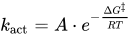
${\displaystyle \Delta G^{\ddagger }}$ is the Gibbs free energy of the formation of the transition state, the exponential term represents the probability of its formation, A contains the probability of crossing from precursor to successor complex.

The consequence of an electron transfer is the rearrangement of charges, and this greatly influences the solvent environment. For the dipolar solvent molecules rearrange in the direction of the field of the charges (this is called orientation polarisation), and also the atoms and electrons in the solvent molecules are slightly displaced (atomic and electron polarization, respectively). It is this solvent polarization which determines the free energy of activation and thus the reaction rate.

Substitution, elimination and isomerization reactions differ from the outer sphere redox reaction not only in the structural changes outlined above, but also in the fact that the movements of the nuclei and the shift of charges (charge transfer, CT) on the reactions path take place in a continuous and concerted way: nuclear configurations and charge distribution are always "in equilibrium". This is illustrated by the S_N2 substitution of the saponification of an alkyl halide where the rear side attack of the OH⁻ ion pushes out a halide ion and where a transition state with a five-coordinated carbon atom must be visualized. The system of the reactants becomes coupled so tightly during the reaction that they form the activated complex as an integral entity. The solvent here has a minor effect.

By contrast, in outer sphere redox reactions the displacement of nuclei in the reactants are small, here the solvent has the dominant role. Donor-acceptor coupling is weak, both keep their identity during the reaction. Therefore, the electron, being an elementary particle, can only "jump" as a whole (electron transfer, ET). If the electron jumps, the transfer is much faster than the movement of the large solvent molecules, with the consequence that the nuclear positions of the reaction partners and the solvent molecules are the same before and after the electron jump (Franck–Condon principle).^[7] The jump of the electron is governed by quantum mechanical rules, it is only possible if also the energy of the ET system does not change "during" the jump.

The arrangement of solvent molecules depends on the charge distribution on the reactants. If the solvent configuration must be the same before and after the jump and the energy may not change, then the solvent cannot be in the solvation state of the precursor nor in that of the successor complex as they are different, it has to be somewhere in between. For the self-exchange reaction for symmetry reasons an arrangement of the solvent molecules exactly in the middle of those of precursor and successor complex would meet the conditions. This means that the solvent arrangement with half of the electron on both donor and acceptor would be the correct environment for jumping. Also, in this state the energy of precursor and successor in their solvent environment would be the same.

However, the electron as an elementary particle cannot be divided, it resides either on the donor or the acceptor and arranges the solvent molecules accordingly in an equilibrium. The "transition state", on the other hand, requires a solvent configuration which would result from the transfer of half an electron, which is impossible. This means that real charge distribution and required solvent polarization are not in an "equilibrium". Yet it is possible that the solvent takes a configuration corresponding to the "transition state", even if the electron sits on the donor or acceptor. This, however, requires energy. This energy may be provided by the thermal energy of the solvent and thermal fluctuations can produce the correct polarization state. Once this has been reached the electron can jump. The creation of the correct solvent arrangement and the electron jump are decoupled and do not happen in a synchronous process. Thus the energy of the transition state is mostly polarization energy of the solvent.

On the basis of his reasoning R.A. Marcus developed a classical theory with the aim of calculating the polarization energy of the said non-equilibrium state. From thermodynamics it is well known that the energy of such a state can be determined if a reversible path to that state is found. Marcus was successful in finding such a path via two reversible charging steps for the preparation of the "transition state" from the precursor complex.

Four elements are essential for the model on which the theory is based:

1. Marcus employs a classical, purely electrostatic model. The charge (many elementary charges) may be transferred in any portion from one body to another.
2. Marcus separates the fast electron polarisation P_e and the slow atom and orientation polarisation P_u of the solvent on grounds of their time constants differing several orders of magnitude.
3. Marcus separates the inner sphere (reactant + tightly bound solvent molecules, in complexes + ligands) and the outer sphere (free solvent )
4. In this model Marcus confines himself to calculating the outer sphere energy of the non-equilibrium polarization of the "transition state". The outer sphere energy is often much larger than the inner sphere contribution because of the far reaching electrostatic forces (compare the Debye–Hückel theory of electrochemistry).

Marcus' tool is the theory of dielectric polarization in solvents. He solved the problem in a general way for a transfer of charge between two bodies of arbitrary shape with arbitrary surface and volume charge. For the self-exchange reaction, the redox pair (e.g. Fe(H₂O)₆³⁺ / Fe(H₂O)₆²⁺) is substituted by two macroscopic conducting spheres at a defined distance carrying specified charges. Between these spheres a certain amount of charge is reversibly exchanged.

In the first step the energy W_I of the transfer of a specific amount of charge is calculated, e.g. for the system in a state when both spheres carry half of the amount of charge which is to be transferred. This state of the system can be reached by transferring the respective charge from the donor sphere to the vacuum and then back to the acceptor sphere.^[8] Then the spheres in this state of charge give rise to a defined electric field in the solvent which creates the total solvent polarization P_u + P_e. By the same token this polarization of the solvent interacts with the charges.

In a second step the energy W_II of the reversible (back) transfer of the charge to the first sphere, again via the vacuum, is calculated. However, the atom and orientation polarization P_u is kept fixed, only the electron polarization P_e may adjust to the field of the new charge distribution and the fixed P_u. After this second step the system is in the desired state with an electron polarization corresponding to the starting point of the redox reaction and an atom and orientation polarization corresponding to the "transition state". The energy W_I + W_II of this state is, thermodynamically speaking, a Gibbs free energy G.

Of course, in this classical model the transfer of any arbitrary amount of charge Δe is possible. So the energy of the non-equilibrium state, and consequently of the polarization energy of the solvent, can be probed as a function of Δe. Thus Marcus has lumped together, in a very elegant way, the coordinates of all solvent molecules into a single coordinate of solvent polarization Δp which is determined by the amount of transferred charge Δe. So he reached a simplification of the energy representation to only two dimensions: G = f(Δe). The result for two conducting spheres in a solvent is the formula of Marcus

${\displaystyle G=\left({\frac {1}{2r_{1}}}+{\frac {1}{2r_{2}}}-{\frac {1}{R}}\right)\cdot \left({\frac {1}{\epsilon _{\text{opt}}}}-{\frac {1}{\epsilon _{\text{s}}}}\right)\cdot (\Delta e)^{2}}$

Where r₁ and r₂ are the radii of the spheres and R is their separation, ε_s and ε_opt are the static and high frequency (optical) dielectric constants of the solvent, Δe the amount of charge transferred. The graph of G vs. Δe is a parabola (Fig. 1). In Marcus theory the energy belonging to the transfer of a unit charge (Δe = 1) is called the (outer sphere) reorganization energy λ_o, i.e. the energy of a state where the polarization would correspond to the transfer of a unit amount of charge, but the real charge distribution is that before the transfer.^[9] In terms of exchange direction the system is symmetric.

Shrinking the two-sphere model to the molecular level creates the problem that in the self-exchange reaction the charge can no longer be transferred in arbitrary amounts, but only as a single electron. However, the polarization still is determined by the total ensemble of the solvent molecules and therefore can still be treated classically, i.e. the polarization energy is not subject to quantum limitations. Therefore, the energy of solvent reorganization can be calculated as being due to a hypothetical transfer and back transfer of a partial elementary charge according to the Marcus formula. Thus the reorganization energy for chemical redox reactions, which is a Gibbs free energy, is also a parabolic function of Δe of this hypothetical transfer, For the self exchange reaction, where for symmetry reasons Δe = 0.5, the Gibbs free energy of activation is ΔG(0)^‡ = λ_o/4 (see Fig. 1 and Fig. 2 intersection of the parabolas I and f, f(0), respectively).

Up to now all was physics, now some chemistry enters. The self exchange reaction is a very specific redox reaction, most of the redox reactions are between different partners^[10] e.g.

${\displaystyle {\ce {{[Fe^{II}(CN)6]^{4-}}+{[Ir^{IV}Cl6]^{2-}}<=>{[Fe^{III}(CN)6]^{3-}}+{[Ir^{III}Cl6]^{3-}}}}}$

and they have positive (endergonic) or negative (exergonic) Gibbs free energies of reaction ${\displaystyle \Delta G^{\circ }}$.

As Marcus calculations refer exclusively to the electrostatic properties in the solvent (outer sphere) ${\displaystyle \Delta G^{\circ }}$ and ${\displaystyle \lambda _{0}}$ are independent of one another and therefore can just be added up. This means that the Marcus parabolas in systems with different ${\displaystyle \Delta G^{\circ }}$ are shifted just up or down in the ${\displaystyle G}$ vs. ${\displaystyle \Delta e}$ diagram (Fig. 2). Variation of ${\displaystyle \Delta G^{\circ }}$ can be affected in experiments by offering different acceptors to the same donor.

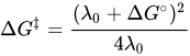
Simple calculation of the intersection point between the parabolas i ${\displaystyle (y=x^{2})}$ and ${\displaystyle f_{i}}$ ${\displaystyle (y=(x-d)^{2}+c)}$ give the Gibbs free energy of activation

${\displaystyle \Delta G^{\ddagger }={\frac {(\lambda _{0}+\Delta G^{\circ })^{2}}{4\lambda _{0}}}}$,

where ${\displaystyle \lambda _{0}}$ = ${\displaystyle d^{2}}$ and ${\displaystyle \Delta G^{\circ }}$= c. The intersection of those parabolas represents an activation energy and not the energy of a transition state of fixed configuration of all nuclei in the system as is the case in the substitution and other reactions mentioned. The transition state of the latter reactions has to meet structural and energetic conditions, redox reactions have only to comply to the energy requirement. Whereas the geometry of the transition state in the other reactions is the same for all pairs of reactants, for redox pairs many polarization environments may meet the energetic conditions.

Marcus' formula shows a quadratic dependence of the Gibbs free energy of activation on the Gibbs free energy of reaction. It is general knowledge from the host of chemical experience that reactions usually are the faster the more negative is ${\displaystyle \Delta G^{\circ }}$. In many cases even a linear free energy relation is found. According to the Marcus formula the rates increase also when the reactions are more exergonic, however only as long as ${\displaystyle \Delta G^{\circ }}$ is positive or slightly negative. It is surprising that for redox reactions according to the Marcus formula the activation energy should increase for very exergonic reaction, i.e. in the cases when ${\displaystyle \Delta G^{\circ }}$ is negative and its absolute value is greater than that of ${\displaystyle \lambda _{0}}$. This realm of Gibbs free energy of reaction is called "Marcus inverted region". In Fig. 2 it becomes obvious that the intersection of the parabolas i and f moves upwards in the left part of the graph when ${\displaystyle \Delta G^{\circ }}$ continues to become more negative, and this means increasing activation energy. Thus the total graph of ${\displaystyle \ln k}$ vs. ${\displaystyle \Delta G^{\circ }}$ should have a maximum.

The maximum of the ET rate is expected at ${\displaystyle \Delta G^{\ddagger }=0.}$ Here ${\displaystyle \Delta e=0}$ and ${\displaystyle q=0}$ (Fig. 2) which means that the electron may jump in the precursor complex at its equilibrium polarization. No thermal activation is necessary: the reaction is barrierless. In the inverted region the polarization corresponds to the difficult-to-imagine notion of a charge distribution where the donor has received and the acceptor given off charge. Of course, in real world this does not happen, it is not a real charge distribution which creates this critical polarization, but the thermal fluctuation in the solvent. This polarization necessary for transfer in the inverted region can be created – with some probability – as well as any other one.^[11] The electron is just waiting for it for jumping.

In the outer sphere model the donor or acceptor and the tightly bound solvation shells or the complex' ligands were considered to form rigid structures which do not change in the course of electron transfer. However, the distances in the inner sphere are dependent on the charge of donor and acceptor, e.g., the central ion-ligand distances are different in complexes carrying different charges and again the Franck–Condon principle must be obeyed: for the electron to jump to occur, the nuclei have to have an identical configuration to both the precursor and the successor complexes, of course highly distorted. In this case the energy requirement is fulfilled automatically.

In this inner sphere case the Arrhenius concept holds, the transition state of definite geometric structure is reached along a geometrical reaction coordinate determined by nuclear motions. No further nuclear motion is necessary to form the successor complex, just the electron jumps, which makes a difference to the TST theory. The reaction coordinate for inner sphere energy is governed by vibrations and they differ in the oxidized and reduced species.^[12]

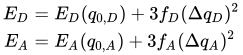
For the self-exchange system Fe²⁺/Fe³⁺ only the symmetrical breathing vibration of the six water molecules around the iron ions is considered.^[12] Assuming harmonic conditions this vibration has frequencies ${\displaystyle \nu _{D}}$ and ${\displaystyle \nu _{A}}$, the force constants ${\displaystyle f_{D}}$ and ${\displaystyle f_{A}}$ are ${\displaystyle f=4\pi ^{2}\nu ^{2}\mu }$ and the energies are

${\displaystyle {\begin{aligned}E_{D}&=E_{D}(q_{0,D})+3f_{D}(\Delta q_{D})^{2}\\E_{A}&=E_{A}(q_{0,A})+3f_{A}(\Delta q_{A})^{2}\end{aligned}}}$

where ${\displaystyle q_{0}}$ is the equilibrium normal coordinate and ${\displaystyle \Delta q=(q-q_{0})}$ the displacement along the normal coordinate, the factor 3 stems from 6 (H₂O)·1⁄2. Like for the outer-sphere reorganization energy potential energy curve is quadratic, here, however, as a consequence of vibrations.

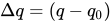
The equilibrium normal coordinates differ in Fe(H₂O)₆²⁺ and Fe(H₂O)₆³⁺. By thermal excitation of the breathing vibration a geometry can be reached which is common to both donor and acceptor, i.e., the potential energy curves of the breathing vibrations of D and A intersect here. This is the situation where the electron may jump. The energy of this transition state is the inner sphere reorganization energy ${\displaystyle \lambda _{\text{in}}}$.

For the self-exchange reaction the metal-water distance in the transition state can be calculated^[12]

${\displaystyle q^{*}={\frac {f_{D}q_{0,D}+f_{A}q_{0,A}}{f_{D}+f_{A}}}}$

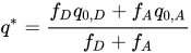
This gives the inner sphere reorganisation energy

${\displaystyle \lambda _{\text{in}}=\Delta E^{*}={\frac {3f_{D}f_{A}}{f_{D}+f_{A}}}(q_{0,D}-q_{0,A})^{2}}$

It is fortunate that the expressions for the energies for outer and inner reorganization have the same quadratic form. Inner sphere and outer sphere reorganization energies are independent, so they can be added to give ${\displaystyle \lambda =\lambda _{\text{in}}+\lambda _{o}}$ and inserted in the Arrhenius equation

${\displaystyle k_{\text{act}}=A\cdot e^{-{\frac {\Delta {G_{\text{in}}^{\ddagger }}+\Delta {G_{o}}^{\ddagger }}{kT}}}}$

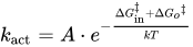
Here, ${\displaystyle A}$ can be seen to represent the probability of electron jump, exp[-ΔG_in^‡/kT] that of reaching the transition state of the inner sphere and exp[-ΔG_o^‡/kT] that of outer sphere adjustment.

For unsymmetrical (cross) reactions like

${\displaystyle {\ce {{[Fe(H2O)6]^{2}+}+{[Co(H2O)6]^{3}+}<=>{[Fe(H2O)6]^{3}+}+{[Co(H2O)6]^{2}+}}}}$

the expression for ${\displaystyle \lambda _{in}}$ can also be derived, but it is more complicated.^[12] These reactions have a free reaction enthalpy ${\displaystyle \Delta G^{0}}$ which is independent of the reorganization energy and determined by the different redox potentials of the iron and cobalt couple. Consequently, the quadratic Marcus equation holds also for the inner sphere reorganization energy, including the prediction of an inverted region. One may visualizing this by (a) in the normal region both the initial state and the final state have to have stretched bonds, (b) In the ${\displaystyle \Delta G^{\ddagger }=0}$ case the equilibrium configuration of the initial state is the stretched configuration of the final state, and (c) in the inverted region the initial state has compressed bonds whereas the final state has largely stretched bonds. Similar considerations hold for metal complexes where the ligands are larger than solvent molecules and also for ligand bridged polynuclear complexes.

The strength of the electronic coupling of the donor and acceptor decides whether the electron transfer reaction is adiabatic or non-adiabatic. In the non-adiabatic case the coupling is weak, i.e. H_AB in Fig. 3 is small compared to the reorganization energy and donor and acceptor retain their identity. The system has a certain probability to jump from the initial to the final potential energy curves. In the adiabatic case the coupling is considerable, the gap of 2 H_AB is larger and the system stays on the lower potential energy curve.^[13]

Marcus theory as laid out above, represents the non-adiabatic case.^[14] Consequently, the semi-classical Landau-Zener theory can be applied, which gives the probability of interconversion of donor and acceptor for a single passage of the system through the region of the intersection of the potential energy curves

${\displaystyle P_{if}=1-\exp \left[-{\frac {4\pi ^{2}{H_{if}^{2}}}{hv\left|s_{i}-s_{f}\right|}}\right]}$

where H_if is the interaction energy at the intersection, v the velocity of the system through the intersection region, s_i and s_f the slopes there.

Working this out, one arrives at the basic equation of Marcus theory

${\displaystyle k_{et}={\frac {2\pi }{\hbar }}|H_{AB}|^{2}{\frac {1}{\sqrt {4\pi \lambda k_{\rm {B}}T}}}\exp \left(-{\frac {(\lambda +\Delta G^{\circ })^{2}}{4\lambda k_{\rm {B}}T}}\right)}$

where ${\displaystyle k_{et}}$ is the rate constant for electron transfer, ${\displaystyle |H_{AB}|}$ is the electronic coupling between the initial and final states, ${\displaystyle \lambda }$ is the reorganization energy (both inner and outer-sphere), and ${\displaystyle \Delta G^{\circ }}$ is the total Gibbs free energy change for the electron transfer reaction (${\displaystyle k_{\rm {B}}}$ is the Boltzmann constant and ${\displaystyle T}$ is the absolute temperature).

Thus Marcus's theory builds on the traditional Arrhenius equation for the rates of chemical reactions in two ways: 1. It provides a formula for the activation energy, based on a parameter called the reorganization energy, as well as the Gibbs free energy. The reorganization energy is defined as the energy required to "reorganize" the system structure from initial to final coordinates, without making the charge transfer. 2. It provides a formula for the pre-exponential factor in the Arrhenius equation, based on the electronic coupling between the initial and final state of the electron transfer reaction (i.e., the overlap of the electronic wave functions of the two states).

Marcus published his theory in 1956. For many years there was an intensive search for the inverted region which would be a proof of the theory. But all experiments with series of reactions of more and more negative ΔG⁰ revealed only an increase of the reaction rate up to the diffusion limit, i.e. to a value indicating that every encounter lead to electron transfer, and that limit held also for very negative ΔG⁰ values (Rehm-Weller behaviour).^[15] It took about 30 years until the inverted region was unequivocally substantiated by Miller, Calcaterra and Closs for an intramolecular electron transfer in a molecule where donor and acceptor are kept at a constant distance by means of a stiff spacer (Fig.4).^[16]

A posteriori one may presume that in the systems where the reaction partners may diffuse freely the optimum distance for the electron jump may be sought, i.e. the distance for which ΔG^‡ = 0 and ΔG⁰ = - λ_o. For λ_o is dependent on R, λ_o increases for larger R and the opening of the parabola smaller. It is formally always possible to close the parabola in Fig. 2 to such an extent, that the f-parabola intersects the i-parabola in the apex. Then always ΔG^‡ = 0 and the rate k reaches the maximum diffusional value for all very negative ΔG⁰. There are, however, other concepts for the phenomenon,^[1] e.g. the participation of excited states or that the decrease of the rate constants would be so far in the inverted region that it escapes measurement.

R. A. Marcus and his coworkers have further developed the theory outlined here in several aspects. They have included inter alia statistical aspects and quantum effects,^[17] they have applied the theory to chemiluminescence^[18] and electrode reactions.^[19] R. A. Marcus received the Nobel Prize in Chemistry in 1992, and his Nobel Lecture gives an extensive view of his work.^[1]

• Hammond's postulate
• Solvated electron
• Free-energy relationship

• Marcus, R.A (1956). "On the Theory of Oxidation-Reduction Reactions Involving Electron Transfer. I" (PDF). J. Chem. Phys. 24 (5): 966–978. Bibcode:1956JChPh..24..966M. doi:10.1063/1.1742723. S2CID 16579694.
• Marcus, R.A (1956). "Electrostatic Free Energy and Other Properties of States Having Nonequilibrium Polarization. I" (PDF). J. Chem. Phys. 24 (5): 979–989. Bibcode:1956JChPh..24..979M. doi:10.1063/1.1742724.
• Marcus, R.A (1957). "On the Theory of Oxidation-Reduction Reactions Involving Electron Transfer. II. Applications to Data on the Rates of Isotopic Exchange Reactions" (PDF). J. Chem. Phys. 26 (4): 867–871. Bibcode:1957JChPh..26..867M. doi:10.1063/1.1743423.
• Marcus, R.A (1957). "On the Theory of Oxidation-Reduction Reactions Involving Electron Transfer. III. Applications to Data on the Rates of Organic Redox Reactions" (PDF). J. Chem. Phys. 26 (4): 872–877. Bibcode:1957JChPh..26..872M. doi:10.1063/1.1743424.
• Marcus, R.A (1960). "Exchange reactions and electron transfer reactions including isotopic exchange. Theory of oxidation-reduction reactions involving electron transfer. Part 4.—A statistical-mechanical basis for treating contributions from solvent, ligands, and inert salt" (PDF). Discuss. Faraday Soc. 29: 21–31. doi:10.1039/df9602900021.
• Marcus, R.A (1963). "On The Theory Of Oxidation--Reduction Reactions Involving Electron Transfer. V. Comparison And Properties Of Electrochemical And Chemical Rate Constants". J. Phys. Chem. 67 (4): 853–857. doi:10.1021/j100798a033. OSTI 4712863.
• Marcus, R.A (1964). "Chemical and Electrochemical Electron-Transfer Theory". Annu. Rev. Phys. Chem. 15 (1): 155–196. Bibcode:1964ARPC...15..155M. doi:10.1146/annurev.pc.15.100164.001103.
• Marcus, R.A (1965). "On the Theory of Electron-Transfer Reactions. VI. Unified Treatment for Homogeneous and Electrode Reactions" (PDF). J. Chem. Phys. 43 (2): 679–701. Bibcode:1965JChPh..43..679M. doi:10.1063/1.1696792.
• Marcus, R.A.; Sutin N (1985). "Electron transfers in chemistry and biology". Biochim. Biophys. Acta. 811 (3): 265. doi:10.1016/0304-4173(85)90014-X.