Marginal product

Marginal productMain

Community hub

Marginal product

8 pages, 0 posts

0 subscribers

Recent from talks

Be the first to start a discussion here.

Recent from talks

Be the first to start a discussion here.

Contribute something

About hubMembersContent overviewUpdatesRules

Main reference articles

Marginal product

View on Wikipedia

from Wikipedia

In economics and in particular neoclassical economics, the marginal product or marginal physical productivity of an input (factor of production) is the change in output resulting from employing one more unit of a particular input (for instance, the change in output when a firm's labor is increased from five to six units), assuming that the quantities of other inputs are kept constant.^[1]

The marginal product of a given input can be expressed^[2] as:

MP={\frac {\Delta Y}{\Delta X}}

where $\Delta X$ is the change in the firm's use of the input (conventionally a one-unit change) and $\Delta Y$ is the change in the quantity of output produced (resulting from the change in the input). Note that the quantity $Y$ of the "product" is typically defined ignoring external costs and benefits.

If the output and the input are infinitely divisible, so the marginal "units" are infinitesimal, the marginal product is the mathematical derivative of the production function with respect to that input. Suppose a firm's output Y is given by the production function:

Y=F(K,L)

where K and L are inputs to production (say, capital and labor, respectively). Then the marginal product of capital (MPK) and marginal product of labor (MPL) are given by:

MPK={\frac {\partial F}{\partial K}}

MPL={\frac {\partial F}{\partial L}}

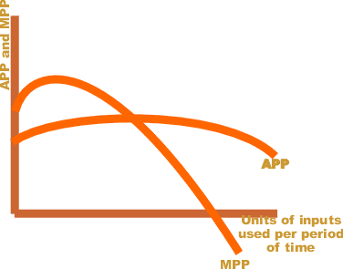
In the law of diminishing marginal returns, the marginal product initially increases when more of an input (say labor) is employed, keeping the other input (say capital) constant. Here, labor is the variable input and capital is the fixed input (in a hypothetical two-inputs model). As more and more of variable input (labor) is employed, marginal product starts to fall. Finally, after a certain point, the marginal product becomes negative, implying that the additional unit of labor has decreased the output, rather than increasing it. The reason behind this is the diminishing marginal productivity of labor.

The marginal product of labor is the slope of the total product curve, which is the production function plotted against labor usage for a fixed level of usage of the capital input.

In the neoclassical theory of competitive markets, the marginal product of labor equals the real wage. In aggregate models of perfect competition, in which a single good is produced and that good is used both in consumption and as a capital good, the marginal product of capital equals its rate of return. As was shown in the Cambridge capital controversy, this proposition about the marginal product of capital cannot generally be sustained in multi-commodity models in which capital and consumption goods are distinguished.^[3]

Relationship of marginal product (MPP) with the total product (TPP)

[edit]

The relationship can be explained in three phases- (1) Initially, as the quantity of variable input is increased, TPP rises at an increasing rate. In this phase, MPP also rises. (2) As more and more quantities of the variable inputs are employed, TPP increases at a diminishing rate. In this phase, MPP starts to fall. (3) When the TPP reaches its maximum, MPP is zero. Beyond this point, TPP starts to fall and MPP becomes negative.

References

[edit]

^ Brewer, Anthony (2010). The Making of the Classical Theory of Economic Growth. Routledge. ISBN 978-0415486200.
^ Mukherjee, Sampat; Mukherjee, Mallinath; Ghose, Amitava (2003). Microeconomics. New Delhi: Prentice-Hall of India. ISBN 81-203-2318-1.
^ Kurz, Heinz D. and Neri Salvadori (1995) Theory of Production: A Long-Period Analysis. Cambridge University Press.

View on Grokipedia

from Grokipedia

In economics, the marginal product of a factor of production—such as labor, capital, or materials—refers to the additional output generated by employing one more unit of that factor while holding all other inputs constant.^[1] This concept is central to understanding how firms transform inputs into outputs through a production function, typically expressed as

Q = f(L, K)

, where

Q

is total output,

L

is labor, and

K

is capital.^[2] The marginal product is calculated as the change in output divided by the change in the input, or

MP = \Delta Q / \Delta X

, where

X

represents the variable input; in continuous terms, it is the partial derivative of the production function with respect to that input.^[2] For example, the marginal product of labor (

MPL

) measures the extra output from one additional worker, assuming fixed capital and technology.^[3] A key feature is the law of diminishing marginal returns, which holds in the short run—when at least one input is fixed—that successive units of a variable input yield progressively smaller increases in output due to constraints like overcrowding or resource limitations.^[4] Initially, marginal product may rise due to specialization, but it eventually declines, flattening the slope of the production function.^[2] Marginal product plays a crucial role in firm decision-making, particularly in profit maximization, where businesses hire inputs up to the point where the value of the marginal product equals the input's cost—for labor, this means wage equals the marginal revenue product in competitive markets.^[3] In imperfectly competitive settings, it influences employment levels by equating wage to the marginal revenue product, often resulting in lower hiring than in perfect competition.^[3] In the long run, with all inputs variable, marginal products guide cost minimization along isoquants, where the optimal input mix occurs when the ratio of marginal products equals the ratio of input prices, affecting scale and efficiency.^[4] Diminishing marginal returns also underpin rising marginal and average costs, shaping supply curves and market dynamics.^[4]

Definition and Formulation

Core Definition

The marginal product of an input, such as labor or capital, refers to the additional output produced by employing one more unit of that variable input while holding all other inputs constant.^[1] This concept, often denoted in economic analysis as the marginal product of labor (MPL) or marginal product of capital (MPK), measures the incremental contribution of the extra input to total production in the short run, where at least one factor remains fixed.^[5] The idea of marginal product traces its origins to classical economics in the 19th century, with significant development by American economist John Bates Clark in the late 1800s as part of the neoclassical revolution.^[6] Clark's seminal work, The Distribution of Wealth (1899), formalized marginal productivity theory, arguing that factors of production receive remuneration equal to their marginal contributions to output under competitive conditions, building on earlier ideas from economists like John Stuart Mill.^[7] This framework shifted economic thought from labor theories of value toward a productivity-based explanation of income distribution.^[6] Marginal product typically focuses on the marginal physical product, which quantifies the physical increase in output units, distinct from the marginal revenue product that incorporates the monetary value of that output by multiplying the physical increment by the marginal revenue from selling additional units.^[8] For instance, in agriculture, the marginal physical product of labor might manifest as the extra bushels of crops harvested when one additional worker is added to a fixed plot of land, assuming tools and weather remain unchanged.^[9]

Mathematical Formulation

The marginal product of an input, such as labor, measures the additional output produced by employing one more unit of that input, holding all other factors constant. In discrete terms, it is formulated as the ratio of the change in total product to the change in the input level:

\text{MP} = \frac{\Delta \text{TP}}{\Delta L}

where TP denotes total product (output) and L represents the units of the variable input, such as labor. This formulation applies in scenarios where inputs are adjusted in whole units, common in empirical production analysis.^[10] In continuous models, the marginal product is the derivative of the total product with respect to the input:

\text{MP} = \frac{d \text{TP}}{d L}

This captures the instantaneous rate of change in output as the input varies smoothly. For production processes modeled with multiple inputs, the marginal product of labor (MP_L) derives from the total production function Q = f(L, K), where K is fixed capital:

\text{MP}_L = \frac{\partial Q}{\partial L}

This partial derivative assumes ceteris paribus conditions, with other inputs held constant to isolate the effect of the variable input. The short-run context typically features one variable input, such as labor, while capital remains fixed, reflecting real-world constraints like plant capacity.^[11]^[12] To illustrate the discrete formula, consider a firm where total output increases from 100 units to 115 units upon hiring one additional worker, raising labor from 5 to 6 units; the marginal product is then (115 - 100) / (6 - 5) = 15 units per worker. This calculation highlights how marginal product quantifies incremental productivity contributions under fixed other factors.^[10]

Relationships to Production Measures

Connection to Total Product

The total product (TP) represents the overall output resulting from varying levels of a variable input, such as labor, while holding other inputs fixed. It is mathematically equivalent to the cumulative sum of all marginal products (MP) up to the current input level, expressed as

TP = \sum MP

.^[13] This summation illustrates how each successive unit of input contributes incrementally to the aggregate production. Additionally, the marginal product serves as the slope of the total product curve, indicating the rate of change in TP with respect to the input. As long as the marginal product remains positive, the total product curve rises, reflecting ongoing additions to output from each new unit of input. When MP equals zero, total product reaches its maximum, as further input yields no additional output. If MP becomes negative, total product begins to decline, as the extra input detracts from overall efficiency due to overcrowding or resource constraints.^[14]^[13] In the short run, the total product curve typically exhibits an S-shape, starting with an initial concave-up portion driven by increasing marginal returns—where MP rises, causing TP to accelerate upward—followed by a concave-down segment from diminishing marginal returns, where MP falls but remains positive, slowing the TP increase before it plateaus.^[14] This S-shaped trajectory culminates at the point where MP crosses zero, marking the short-run maximum of TP.^[14]

Connection to Average Product

The average product (AP) of labor is defined as the total product (TP) divided by the number of labor units (L), expressed mathematically as

AP = \frac{TP}{L}

. This measure represents the output per unit of labor on average. The marginal product (MP) interacts dynamically with AP, influencing its trajectory as additional labor is employed.^[13]^[15] When MP exceeds AP, the addition of labor raises the AP because the new worker contributes more output than the existing average. Conversely, when MP falls below AP, the AP declines as the additional labor pulls down the overall average productivity. This relationship holds because MP reflects the incremental contribution that "pulls" the average up or down relative to its current level.^[13]^[16]^[15] Graphically, the MP curve intersects the AP curve at the point where AP reaches its maximum, marking the highest average efficiency. At this crossover, MP equals AP, after which diminishing returns typically cause MP to fall below AP, leading to a decline in AP. For instance, suppose the current AP is 20 units per worker; if the next worker's MP is 25 units, adding them increases AP above 20, but if MP is only 15 units, AP drops below 20.^[13]^[16]^[15]

Stages of Production and Returns

Increasing Marginal Returns

Increasing marginal returns refer to the initial stage in the production process where the addition of successive units of a variable input, such as labor, to fixed inputs results in an increasing marginal product.^[17] This phenomenon arises because the additional input enhances the efficiency of the fixed factors, leading to greater output increments per unit added.^[13] The primary causes of increasing marginal returns include worker specialization and improved coordination among inputs during the early stages of production expansion.^[17] As more workers are employed, they can divide tasks more effectively, allowing each to focus on specific aspects of production that leverage their developing skills and reduce idle time for fixed resources like machinery or land.^[13] This division of labor fosters better utilization of the production setup, amplifying the productivity gains from each new input unit. Key characteristics of this stage include a total product curve that rises at an accelerating rate, appearing concave upward, while the marginal product curve ascends toward its maximum point.^[13] In mathematical terms, this corresponds to a positive second derivative of the total product function with respect to the variable input.^[18] A seminal historical example illustrating increasing marginal returns through specialization is Adam Smith's description of a pin factory in The Wealth of Nations.^[19] Smith observed that a single worker, unskilled in pin-making, might produce only one pin per day, but when ten workers specialized in distinct operations—such as drawing wire or cutting heads—their combined output reached nearly 48,000 pins daily, vastly elevating the marginal product per worker due to the efficiencies of divided labor.^[19]

Diminishing Marginal Returns

The law of diminishing marginal returns states that, beyond a certain point in the production process, the addition of successive units of a variable input to fixed factors of production will yield progressively smaller increases in output, holding all else constant (ceteris paribus).^[20] This principle assumes that at least one factor, such as land or capital, remains fixed while the variable input, like labor, is increased. This concept was originally formulated by David Ricardo in the early 19th century as part of his theory of rent, where it explained declining productivity in agriculture as more labor and capital were applied to fixed land supplies of varying fertility.^[21]^[20] Ricardo's analysis, detailed in his 1817 work On the Principles of Political Economy and Taxation, highlighted how additional inputs on inferior lands or intensified cultivation on fixed plots led to reduced marginal yields, influencing rising rents and food prices during the Napoleonic era.^[21] In modern economics, the law extends beyond agriculture to general production scenarios, emphasizing its role in resource allocation.^[20] The primary causes of diminishing marginal returns stem from the constraints imposed by fixed inputs, which eventually become bottlenecks as variable inputs accumulate. For instance, overcrowding occurs when too many workers share limited machinery or space, reducing each worker's efficiency due to interference, resource strain, or suboptimal coordination. Similarly, in agriculture, excessive labor on fixed land plots can lead to soil exhaustion or inefficient tool usage, diminishing the additional output per worker.^[20] In the progression of production stages, diminishing marginal returns follow the initial phase of increasing returns, where marginal product rises due to better utilization of fixed factors. During this diminishing phase, marginal product remains positive but falls continuously as more variable input is added, reflecting the law's core effect. If inputs continue to increase unchecked, marginal product eventually turns negative, marking a stage where total output declines due to severe inefficiencies like total overcrowding. This sequence underscores the importance of optimal input levels to avoid wasteful overextension.^[20]

Applications in Economic Analysis

Role in Cost Theory

In cost theory, the marginal product of labor (MP_L) plays a central role in deriving the marginal cost (MC) of production, particularly for variable inputs like labor. Specifically, when labor is the only variable input, MC equals the wage rate (w) divided by MP_L, expressed as MC = w / MP_L.^[22]^[23] This formula arises because the cost of producing an additional unit of output is the cost of the additional labor required, adjusted by how much output that labor produces. This relationship highlights an inverse connection between MP_L and MC: as MP_L increases, MC decreases, and vice versa. When MP_L diminishes—due to the law of diminishing marginal returns—more units of labor are needed to produce each additional unit of output, thereby raising the marginal cost per unit.^[24]^[25] The typical U-shaped marginal cost curve emerges from the hump-shaped pattern of the marginal product curve, where MP_L first rises (leading to falling MC) before eventually falling (causing MC to rise). This shape reflects the transition from increasing to diminishing marginal productivity in the short run.^[26]^[27] For instance, in manufacturing, a firm adding workers to an assembly line may initially see rising MP_L from specialization, lowering MC, but as overcrowding sets in and MP_L diminishes, the MC curve steepens, making higher output levels more expensive per unit.^[24]

Firm Production Decisions

Firms maximize profits by adjusting input levels until the marginal revenue product (MRP) of each input equals its price. The MRP represents the additional revenue generated by employing one more unit of an input, calculated as the marginal product (MP) of the input multiplied by the marginal revenue from the extra output it produces: MRP = MP × MR. In perfectly competitive markets, where firms are price takers, marginal revenue equals the product price (P), simplifying the formula to MRP = MP × P. For labor, this implies hiring additional workers until the MRP of labor (MRP_L) equals the wage rate (w), ensuring that the revenue from their output just covers their cost. Similarly, for capital, firms employ it until MRP_K = r, where r is the rental price of capital. This rule stems from the profit-maximization condition that no further gains occur when the value of the last unit's contribution matches its expense.^[28]^[29] In the short run, with some inputs fixed, firms evaluate production levels based on whether additional variable inputs increase output sufficiently to cover costs. Production should halt if the marginal product turns negative, as employing more of the variable input would reduce total output while still incurring variable costs, exacerbating losses beyond the unavoidable fixed costs. This decision aligns with the shutdown rule in competitive markets, where output ceases if price falls below average variable cost, but the negative MP threshold provides a clear signal of inefficiency in input use. By stopping before this point, firms avoid the irrational outcome of diminishing total product, preserving resources for alternative uses.^[30]^[31] In the long run, when all inputs are variable, firms optimize their production process by adjusting combinations to achieve technical efficiency, equalizing the marginal product per dollar spent across inputs. This condition, MP_L / w = MP_K / r, ensures that the last dollar spent on each input yields the same additional output, minimizing costs for any given production level along an isoquant. Failure to equalize these ratios would allow reallocation—such as substituting toward the input with higher MP per dollar—to lower costs without changing output. This adjustment supports overall profit maximization by enabling scalable, efficient expansion or contraction in response to market conditions.^[32]^[33] In competitive markets, firms expand output where the marginal product contributes to covering variable costs, as reflected in the marginal cost curve derived from MP (MC = w / MP_L, assuming labor is the variable input). Production continues as long as the product price exceeds or equals this MC, ensuring that the revenue from additional units, tied to their MP, offsets input expenses. This approach integrates marginal product into output decisions, preventing overproduction and aligning with broader cost theory principles.^[34]

Authority control databases
National	United States France BnF data Israel
Other	Yale LUX

Info Pages

Talk Pages

Special Pages

Marginal product

Recent from talks

Recent from talks

Contribute something

Contribute something

Media Pages

Timelines

Articles

Notes collections

Notes

Notes

Days in Chronicle

Marginal product

Relationship of marginal product (MPP) with the total product (TPP)

See also

References

Further reading