A computational problem can be viewed as an infinite collection of instances together with a set (possibly empty) of solutions for every instance. The input string for a computational problem is referred to as a problem instance, and should not be confused with the problem itself. In computational complexity theory, a problem refers to the abstract question to be solved. In contrast, an instance of this problem is a rather concrete utterance, which can serve as the input for a decision problem. For example, consider the problem of primality testing. The instance is a number (e.g., 15) and the solution is "yes" if the number is prime and "no" otherwise (in this case, 15 is not prime and the answer is "no"). Stated another way, the instance is a particular input to the problem, and the solution is the output corresponding to the given input.

To further highlight the difference between a problem and an instance, consider the following instance of the decision version of the travelling salesman problem: Is there a route of at most 2000 kilometres passing through all of Germany's 14 largest cities? The quantitative answer to this particular problem instance is of little use for solving other instances of the problem, such as asking for a round trip through 14 sites in Milan whose total length is at most 10 km. For this reason, complexity theory addresses computational problems and not particular problem instances.

When considering computational problems, a problem instance is a string over an alphabet. Usually, the alphabet is taken to be the binary alphabet (i.e., the set {0,1}), and thus the strings are bitstrings. As in a real-world computer, mathematical objects other than bitstrings must be suitably encoded. For example, integers can be represented in binary notation, and graphs can be encoded directly via their adjacency matrices, or by encoding their adjacency lists in binary.

Even though some proofs of complexity-theoretic theorems regularly assume some concrete choice of input encoding, one tries to keep the discussion abstract enough to be independent of the choice of encoding. This can be achieved by ensuring that different representations can be transformed into each other efficiently.

Decision problems are one of the central objects of study in computational complexity theory. A decision problem is a type of computational problem where the answer is either yes or no (alternatively, 1 or 0). A decision problem can be viewed as a formal language, where the members of the language are instances whose output is yes, and the non-members are those instances whose output is no. The objective is to decide, with the aid of an algorithm, whether a given input string is a member of the formal language under consideration. If the algorithm deciding this problem returns the answer yes, the algorithm is said to accept the input string, otherwise it is said to reject the input.

An example of a decision problem is the following. The input is an arbitrary graph. The problem consists in deciding whether the given graph is connected or not. The formal language associated with this decision problem is then the set of all connected graphs—to obtain a precise definition of this language, one has to decide how graphs are encoded as binary strings.

A function problem is a computational problem where a single output (of a total function) is expected for every input, but the output is more complex than that of a decision problem—that is, the output is not just yes or no. Notable examples include the traveling salesman problem and the integer factorization problem.

It is tempting to think that the notion of function problems is much richer than the notion of decision problems. However, this is not really the case, since function problems can be recast as decision problems. For example, the multiplication of two integers can be expressed as the set of triples ${\displaystyle (a,b,c)}$ such that the relation ${\displaystyle a\times b=c}$ holds. Deciding whether a given triple is a member of this set corresponds to solving the problem of multiplying two numbers.

To measure the difficulty of solving a computational problem, one may wish to see how much time the best algorithm requires to solve the problem. However, the running time may, in general, depend on the instance. In particular, larger instances will require more time to solve. Thus the time required to solve a problem (or the space required, or any measure of complexity) is calculated as a function of the size of the instance. The input size is typically measured in bits. Complexity theory studies how algorithms scale as input size increases. For instance, in the problem of finding whether a graph is connected, how much more time does it take to solve a problem for a graph with ${\displaystyle 2n}$ vertices compared to the time taken for a graph with ${\displaystyle n}$ vertices?

If the input size is ${\displaystyle n}$, the time taken can be expressed as a function of ${\displaystyle n}$. Since the time taken on different inputs of the same size can be different, the worst-case time complexity ${\displaystyle T(n)}$ is defined to be the maximum time taken over all inputs of size ${\displaystyle n}$. If ${\displaystyle T(n)}$ is a polynomial in ${\displaystyle n}$, then the algorithm is said to be a polynomial time algorithm. Cobham's thesis argues that a problem can be solved with a feasible amount of resources if it admits a polynomial-time algorithm.

A Turing machine is a mathematical model of a general computing machine. It is a theoretical device that manipulates symbols contained on a strip of tape. Turing machines are not intended as a practical computing technology, but rather as a general model of a computing machine—anything from an advanced supercomputer to a mathematician with a pencil and paper. It is believed that if a problem can be solved by an algorithm, there exists a Turing machine that solves the problem. Indeed, this is the statement of the Church–Turing thesis. Furthermore, it is known that everything that can be computed on other models of computation known to us today, such as a RAM machine, Conway's Game of Life, cellular automata, lambda calculus or any programming language can be computed on a Turing machine. Since Turing machines are easy to analyze mathematically, and are believed to be as powerful as any other model of computation, the Turing machine is the most commonly used model in complexity theory.

Many types of Turing machines are used to define complexity classes, such as deterministic Turing machines, probabilistic Turing machines, non-deterministic Turing machines, quantum Turing machines, symmetric Turing machines and alternating Turing machines. They are all equally powerful in principle, but when resources (such as time or space) are bounded, some of these may be more powerful than others.

A deterministic Turing machine is the most basic Turing machine, which uses a fixed set of rules to determine its future actions. A probabilistic Turing machine is a deterministic Turing machine with an extra supply of random bits. The ability to make probabilistic decisions often helps algorithms solve problems more efficiently. Algorithms that use random bits are called randomized algorithms. A non-deterministic Turing machine is a deterministic Turing machine with an added feature of non-determinism, which allows a Turing machine to have multiple possible future actions from a given state. One way to view non-determinism is that the Turing machine branches into many possible computational paths at each step, and if it solves the problem in any of these branches, it is said to have solved the problem. Clearly, this model is not meant to be a physically realizable model, it is just a theoretically interesting abstract machine that gives rise to particularly interesting complexity classes. For examples, see non-deterministic algorithm.

Many machine models different from the standard multi-tape Turing machines have been proposed in the literature, for example random-access machines. Perhaps surprisingly, each of these models can be converted to another without providing any extra computational power. The time and memory consumption of these alternate models may vary.^[2] What all these models have in common is that the machines operate deterministically.

However, some computational problems are easier to analyze in terms of more unusual resources. For example, a non-deterministic Turing machine is a computational model that is allowed to branch out to check many different possibilities at once. The non-deterministic Turing machine has very little to do with how we physically want to compute algorithms, but its branching exactly captures many of the mathematical models we want to analyze, so that non-deterministic time is a very important resource in analyzing computational problems.

For a precise definition of what it means to solve a problem using a given amount of time and space, a computational model such as the deterministic Turing machine is used. The time required by a deterministic Turing machine ${\displaystyle M}$ on input ${\displaystyle x}$ is the total number of state transitions, or steps, the machine makes before it halts and outputs the answer ("yes" or "no"). A Turing machine ${\displaystyle M}$ is said to operate within time ${\displaystyle f(n)}$ if the time required by ${\displaystyle M}$ on each input of length ${\displaystyle n}$ is at most ${\displaystyle f(n)}$. A decision problem ${\displaystyle A}$ can be solved in time ${\displaystyle f(n)}$ if there exists a Turing machine operating in time ${\displaystyle f(n)}$ that solves the problem. Since complexity theory is interested in classifying problems based on their difficulty, one defines sets of problems based on some criteria. For instance, the set of problems solvable within time ${\displaystyle f(n)}$ on a deterministic Turing machine is then denoted by DTIME(${\displaystyle f(n)}$).

Analogous definitions can be made for space requirements. Although time and space are the most well-known complexity resources, any complexity measure can be viewed as a computational resource. Complexity measures are very generally defined by the Blum complexity axioms. Other complexity measures used in complexity theory include communication complexity, circuit complexity, and decision tree complexity.

The complexity of an algorithm is often expressed using big O notation.

The best, worst and average case complexity refer to three different ways of measuring the time complexity (or any other complexity measure) of different inputs of the same size. Since some inputs of size ${\displaystyle n}$ may be faster to solve than others, we define the following complexities:

1. Best-case complexity: This is the complexity of solving the problem for the best input of size ${\displaystyle n}$.
2. Average-case complexity: This is the complexity of solving the problem on an average. This complexity is only defined with respect to a probability distribution over the inputs. For instance, if all inputs of the same size are assumed to be equally likely to appear, the average case complexity can be defined with respect to the uniform distribution over all inputs of size ${\displaystyle n}$.
3. Amortized analysis: Amortized analysis considers both the costly and less costly operations together over the whole series of operations of the algorithm.
4. Worst-case complexity: This is the complexity of solving the problem for the worst input of size ${\displaystyle n}$.

The order from cheap to costly is: Best, average (of discrete uniform distribution), amortized, worst.

For example, the deterministic sorting algorithm quicksort addresses the problem of sorting a list of integers. The worst-case is when the pivot is always the largest or smallest value in the list (so the list is never divided). In this case, the algorithm takes time O(${\displaystyle n^{2}}$). If we assume that all possible permutations of the input list are equally likely, the average time taken for sorting is ${\displaystyle O(n\log n)}$. The best case occurs when each pivoting divides the list in half, also needing ${\displaystyle O(n\log n)}$ time.

To classify the computation time (or similar resources, such as space consumption), it is helpful to demonstrate upper and lower bounds on the maximum amount of time required by the most efficient algorithm to solve a given problem. The complexity of an algorithm is usually taken to be its worst-case complexity unless specified otherwise. Analyzing a particular algorithm falls under the field of analysis of algorithms. To show an upper bound ${\displaystyle T(n)}$ on the time complexity of a problem, one needs to show only that there is a particular algorithm with running time at most ${\displaystyle T(n)}$. However, proving lower bounds is much more difficult, since lower bounds make a statement about all possible algorithms that solve a given problem. The phrase "all possible algorithms" includes not just the algorithms known today, but any algorithm that might be discovered in the future. To show a lower bound of ${\displaystyle T(n)}$ for a problem requires showing that no algorithm can have time complexity lower than ${\displaystyle T(n)}$.

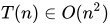
Upper and lower bounds are usually stated using the big O notation, which hides constant factors and smaller terms. This makes the bounds independent of the specific details of the computational model used. For instance, if ${\displaystyle T(n)=7n^{2}+15n+40}$, in big O notation one would write ${\displaystyle T(n)\in O(n^{2})}$.

A complexity class is a set of problems of related complexity. Simpler complexity classes are defined by the following factors:

• The type of computational problem: The most commonly used problems are decision problems. However, complexity classes can be defined based on function problems, counting problems, optimization problems, promise problems, etc.
• The model of computation: The most common model of computation is the deterministic Turing machine, but many complexity classes are based on non-deterministic Turing machines, Boolean circuits, quantum Turing machines, monotone circuits, etc.
• The resource (or resources) that is being bounded and the bound: These two properties are usually stated together, such as "polynomial time", "logarithmic space", "constant depth", etc.

Some complexity classes have complicated definitions that do not fit into this framework. Thus, a typical complexity class has a definition like the following:

The set of decision problems solvable by a deterministic Turing machine within time ${\displaystyle f(n)}$. (This complexity class is known as DTIME(${\displaystyle f(n)}$).)

But bounding the computation time above by some concrete function ${\displaystyle f(n)}$ often yields complexity classes that depend on the chosen machine model. For instance, the language ${\displaystyle \{xx\mid x{\text{ is any binary string}}\}}$ can be solved in linear time on a multi-tape Turing machine, but necessarily requires quadratic time in the model of single-tape Turing machines. If we allow polynomial variations in running time, Cobham-Edmonds thesis states that "the time complexities in any two reasonable and general models of computation are polynomially related" (Goldreich 2008, Chapter 1.2). This forms the basis for the complexity class P, which is the set of decision problems solvable by a deterministic Turing machine within polynomial time. The corresponding set of function problems is FP.

Many important complexity classes can be defined by bounding the time or space used by the algorithm. Some important complexity classes of decision problems defined in this manner are the following:

Resource	Determinism	Complexity class	Resource constraint
Space	Non-Deterministic	NSPACE(${\displaystyle f(n)}$)	${\displaystyle O(f(n))}$
		NL	${\displaystyle O(\log n)}$
		NPSPACE	${\displaystyle O({\text{poly}}(n))}$
		NEXPSPACE	${\displaystyle O(2^{{\text{poly}}(n)})}$
	Deterministic	DSPACE(${\displaystyle f(n)}$)	${\displaystyle O(f(n))}$
		L	${\displaystyle O(\log n)}$
		PSPACE	${\displaystyle O({\text{poly}}(n))}$
		EXPSPACE	${\displaystyle O(2^{{\text{poly}}(n)})}$
Time	Non-Deterministic	NTIME(${\displaystyle f(n)}$)	${\displaystyle O(f(n))}$
		NP	${\displaystyle O({\text{poly}}(n))}$
		NEXPTIME	${\displaystyle O(2^{{\text{poly}}(n)})}$
	Deterministic	DTIME(${\displaystyle f(n)}$)	${\displaystyle O(f(n))}$
		P	${\displaystyle O({\text{poly}}(n))}$
		EXPTIME	${\displaystyle O(2^{{\text{poly}}(n)})}$

Logarithmic-space classes do not account for the space required to represent the problem.

It turns out that PSPACE = NPSPACE and EXPSPACE = NEXPSPACE by Savitch's theorem.

Other important complexity classes include BPP, ZPP and RP, which are defined using probabilistic Turing machines; AC and NC, which are defined using Boolean circuits; and BQP and QMA, which are defined using quantum Turing machines. #P is an important complexity class of counting problems (not decision problems). Classes like IP and AM are defined using Interactive proof systems. ALL is the class of all decision problems.

For the complexity classes defined in this way, it is desirable to prove that relaxing the requirements on (say) computation time indeed defines a bigger set of problems. In particular, although DTIME(${\displaystyle n}$) is contained in DTIME(${\displaystyle n^{2}}$), it would be interesting to know if the inclusion is strict. For time and space requirements, the answer to such questions is given by the time and space hierarchy theorems respectively. They are called hierarchy theorems because they induce a proper hierarchy on the classes defined by constraining the respective resources. Thus there are pairs of complexity classes such that one is properly included in the other. Having deduced such proper set inclusions, we can proceed to make quantitative statements about how much more additional time or space is needed in order to increase the number of problems that can be solved.

More precisely, the time hierarchy theorem states that ${\displaystyle {\mathsf {DTIME}}{\big (}o(f(n)){\big )}\subsetneq {\mathsf {DTIME}}{\big (}f(n)\cdot \log(f(n)){\big )}}$.

The space hierarchy theorem states that ${\displaystyle {\mathsf {DSPACE}}{\big (}o(f(n)){\big )}\subsetneq {\mathsf {DSPACE}}{\big (}f(n){\big )}}$.

The time and space hierarchy theorems form the basis for most separation results of complexity classes. For instance, the time hierarchy theorem tells us that P is strictly contained in EXPTIME, and the space hierarchy theorem tells us that L is strictly contained in PSPACE.

Many complexity classes are defined using the concept of a reduction. A reduction is a transformation of one problem into another problem. It captures the informal notion of a problem being at most as difficult as another problem. For instance, if a problem ${\displaystyle X}$ can be solved using an algorithm for ${\displaystyle Y}$, ${\displaystyle X}$ is no more difficult than ${\displaystyle Y}$, and we say that ${\displaystyle X}$ reduces to ${\displaystyle Y}$. There are many different types of reductions, based on the method of reduction, such as Cook reductions, Karp reductions and Levin reductions, and the bound on the complexity of reductions, such as polynomial-time reductions or log-space reductions.

The most commonly used reduction is a polynomial-time reduction. This means that the reduction process takes polynomial time. For example, the problem of squaring an integer can be reduced to the problem of multiplying two integers. This means an algorithm for multiplying two integers can be used to square an integer. Indeed, this can be done by giving the same input to both inputs of the multiplication algorithm. Thus we see that squaring is not more difficult than multiplication, since squaring can be reduced to multiplication.

This motivates the concept of a problem being hard for a complexity class. A problem ${\displaystyle X}$ is hard for a class of problems ${\displaystyle C}$ if every problem in ${\displaystyle C}$ can be reduced to ${\displaystyle X}$. Thus no problem in ${\displaystyle C}$ is harder than ${\displaystyle X}$, since an algorithm for ${\displaystyle X}$ allows us to solve any problem in ${\displaystyle C}$. The notion of hard problems depends on the type of reduction being used. For complexity classes larger than P, polynomial-time reductions are commonly used. In particular, the set of problems that are hard for NP is the set of NP-hard problems.

If a problem ${\displaystyle X}$ is in ${\displaystyle C}$ and hard for ${\displaystyle C}$, then ${\displaystyle X}$ is said to be complete for ${\displaystyle C}$. This means that ${\displaystyle X}$ is the hardest problem in ${\displaystyle C}$. (Since many problems could be equally hard, one might say that ${\displaystyle X}$ is one of the hardest problems in ${\displaystyle C}$.) Thus the class of NP-complete problems contains the most difficult problems in NP, in the sense that they are the ones most likely not to be in P. Because the problem P = NP is not solved, being able to reduce a known NP-complete problem, ${\displaystyle \Pi _{2}}$, to another problem, ${\displaystyle \Pi _{1}}$, would indicate that there is no known polynomial-time solution for ${\displaystyle \Pi _{1}}$. This is because a polynomial-time solution to ${\displaystyle \Pi _{1}}$ would yield a polynomial-time solution to ${\displaystyle \Pi _{2}}$. Similarly, because all NP problems can be reduced to the set, finding an NP-complete problem that can be solved in polynomial time would mean that P = NP.^[3]

The complexity class P is often seen as a mathematical abstraction modeling those computational tasks that admit an efficient algorithm. This hypothesis is called the Cobham–Edmonds thesis. The complexity class NP, on the other hand, contains many problems that people would like to solve efficiently, but for which no efficient algorithm is known, such as the Boolean satisfiability problem, the Hamiltonian path problem and the vertex cover problem. Since deterministic Turing machines are special non-deterministic Turing machines, it is easily observed that each problem in P is also member of the class NP.

The question of whether P equals NP is one of the most important open questions in theoretical computer science because of the wide implications of a solution.^[3] If the answer is yes, many important problems can be shown to have more efficient solutions. These include various types of integer programming problems in operations research, many problems in logistics, protein structure prediction in biology,^[5] and the ability to find formal proofs of pure mathematics theorems.^[6] The P versus NP problem is one of the Millennium Prize Problems proposed by the Clay Mathematics Institute. There is a US$1,000,000 prize for resolving the problem.^[7]

It was shown by Ladner that if ${\displaystyle {\textsf {P}}\neq {\textsf {NP}}}$ then there exist problems in ${\displaystyle {\textsf {NP}}}$ that are neither in ${\displaystyle {\textsf {P}}}$ nor ${\displaystyle {\textsf {NP}}}$-complete.^[4] Such problems are called NP-intermediate problems. The graph isomorphism problem, the discrete logarithm problem and the integer factorization problem are examples of problems believed to be NP-intermediate. They are some of the very few NP problems not known to be in ${\displaystyle {\textsf {P}}}$ or to be ${\displaystyle {\textsf {NP}}}$-complete.

The graph isomorphism problem is the computational problem of determining whether two finite graphs are isomorphic. An important unsolved problem in complexity theory is whether the graph isomorphism problem is in ${\displaystyle {\textsf {P}}}$, ${\displaystyle {\textsf {NP}}}$-complete, or NP-intermediate. The answer is not known, but it is believed that the problem is at least not NP-complete.^[8] If graph isomorphism is NP-complete, the polynomial time hierarchy collapses to its second level.^[9] Since it is widely believed that the polynomial hierarchy does not collapse to any finite level, it is believed that graph isomorphism is not NP-complete. The best algorithm for this problem, due to László Babai and Eugene Luks has run time ${\displaystyle O(2^{\sqrt {n\log n}})}$ for graphs with ${\displaystyle n}$ vertices, although some recent work by Babai offers some potentially new perspectives on this.^[10]

The integer factorization problem is the computational problem of determining the prime factorization of a given integer. Phrased as a decision problem, it is the problem of deciding whether the input has a prime factor less than ${\displaystyle k}$. No efficient integer factorization algorithm is known, and this fact forms the basis of several modern cryptographic systems, such as the RSA algorithm. The integer factorization problem is in ${\displaystyle {\textsf {NP}}}$ and in ${\displaystyle {\textsf {co-NP}}}$ (and even in UP and co-UP^[11]). If the problem is ${\displaystyle {\textsf {NP}}}$-complete, the polynomial time hierarchy will collapse to its first level (i.e., ${\displaystyle {\textsf {NP}}}$ will equal ${\displaystyle {\textsf {co-NP}}}$). The best known algorithm for integer factorization is the general number field sieve, which takes time ${\displaystyle O(e^{\left({\sqrt[{3}]{\frac {64}{9}}}\right){\sqrt[{3}]{(\log n)}}{\sqrt[{3}]{(\log \log n)^{2}}}})}$^[12] to factor an odd integer ${\displaystyle n}$. However, the best known quantum algorithm for this problem, Shor's algorithm, does run in polynomial time. Unfortunately, this fact doesn't say much about where the problem lies with respect to non-quantum complexity classes.

Many known complexity classes are suspected to be unequal, but this has not been proved. For instance ${\displaystyle {\textsf {P}}\subseteq {\textsf {NP}}\subseteq {\textsf {PP}}\subseteq {\textsf {PSPACE}}}$, but it is possible that ${\displaystyle {\textsf {P}}={\textsf {PSPACE}}}$. If ${\displaystyle {\textsf {P}}}$ is not equal to ${\displaystyle {\textsf {NP}}}$, then ${\displaystyle {\textsf {P}}}$ is not equal to ${\displaystyle {\textsf {PSPACE}}}$ either. Since there are many known complexity classes between ${\displaystyle {\textsf {P}}}$ and ${\displaystyle {\textsf {PSPACE}}}$, such as ${\displaystyle {\textsf {RP}}}$, ${\displaystyle {\textsf {BPP}}}$, ${\displaystyle {\textsf {PP}}}$, ${\displaystyle {\textsf {BQP}}}$, ${\displaystyle {\textsf {MA}}}$, ${\displaystyle {\textsf {PH}}}$, etc., it is possible that all these complexity classes collapse to one class. Proving that any of these classes are unequal would be a major breakthrough in complexity theory.

Along the same lines, ${\displaystyle {\textsf {co-NP}}}$ is the class containing the complement problems (i.e. problems with the yes/no answers reversed) of ${\displaystyle {\textsf {NP}}}$ problems. It is believed^[13] that ${\displaystyle {\textsf {NP}}}$ is not equal to ${\displaystyle {\textsf {co-NP}}}$; however, it has not yet been proven. It is clear that if these two complexity classes are not equal then ${\displaystyle {\textsf {P}}}$ is not equal to ${\displaystyle {\textsf {NP}}}$, since ${\displaystyle {\textsf {P}}={\textsf {co-P}}}$. Thus if ${\displaystyle P=NP}$ we would have ${\displaystyle {\textsf {co-P}}={\textsf {co-NP}}}$ whence ${\displaystyle {\textsf {NP}}={\textsf {P}}={\textsf {co-P}}={\textsf {co-NP}}}$.

Similarly, it is not known if ${\displaystyle {\textsf {L}}}$ (the set of all problems that can be solved in logarithmic space) is strictly contained in ${\displaystyle {\textsf {P}}}$ or equal to ${\displaystyle {\textsf {P}}}$. Again, there are many complexity classes between the two, such as ${\displaystyle {\textsf {NL}}}$ and ${\displaystyle {\textsf {NC}}}$, and it is not known if they are distinct or equal classes.

It is suspected that ${\displaystyle {\textsf {P}}}$ and ${\displaystyle {\textsf {BPP}}}$ are equal. However, it is currently open if ${\displaystyle {\textsf {BPP}}={\textsf {NEXP}}}$.

A problem that can theoretically be solved, but requires impractical and infinite resources (e.g., time) to do so, is known as an intractable problem.^[14] Conversely, a problem that can be solved in practice is called a tractable problem, literally "a problem that can be handled". The term infeasible (literally "cannot be done") is sometimes used interchangeably with intractable,^[15] though this risks confusion with a feasible solution in mathematical optimization.^[16]

Tractable problems are frequently identified with problems that have polynomial-time solutions (${\displaystyle {\textsf {P}}}$, ${\displaystyle {\textsf {PTIME}}}$); this is known as the Cobham–Edmonds thesis. Problems that are known to be intractable in this sense include those that are EXPTIME-hard. If ${\displaystyle {\textsf {NP}}}$ is not the same as ${\displaystyle {\textsf {P}}}$, then NP-hard problems are also intractable in this sense.

However, this identification is inexact: a polynomial-time solution with large degree or large leading coefficient grows quickly, and may be impractical for practical size problems; conversely, an exponential-time solution that grows slowly may be practical on realistic input, or a solution that takes a long time in the worst case may take a short time in most cases or the average case, and thus still be practical. Saying that a problem is not in ${\displaystyle {\textsf {P}}}$ does not imply that all large cases of the problem are hard or even that most of them are. For example, the decision problem in Presburger arithmetic has been shown not to be in ${\displaystyle {\textsf {P}}}$, yet algorithms have been written that solve the problem in reasonable times in most cases. Similarly, algorithms can solve the NP-complete knapsack problem over a wide range of sizes in less than quadratic time and SAT solvers routinely handle large instances of the NP-complete Boolean satisfiability problem.

To see why exponential-time algorithms are generally unusable in practice, consider a program that makes ${\displaystyle 2^{n}}$ operations before halting. For small ${\displaystyle n}$, say 100, and assuming for the sake of example that the computer does ${\displaystyle 10^{12}}$ operations each second, the program would run for about ${\displaystyle 4\times 10^{10}}$ years, which is the same order of magnitude as the age of the universe. Even with a much faster computer, the program would only be useful for very small instances and in that sense the intractability of a problem is somewhat independent of technological progress. However, an exponential-time algorithm that takes ${\displaystyle 1.0001^{n}}$ operations is practical until ${\displaystyle n}$ gets relatively large.

Similarly, a polynomial time algorithm is not always practical. If its running time is, say, ${\displaystyle n^{15}}$, it is unreasonable to consider it efficient and it is still useless except on small instances. Indeed, in practice even ${\displaystyle n^{3}}$ or ${\displaystyle n^{2}}$ algorithms are often impractical on realistic sizes of problems.

Continuous complexity theory can refer to complexity theory of problems that involve continuous functions that are approximated by discretizations, as studied in numerical analysis. One approach to complexity theory of numerical analysis^[17] is information based complexity.

Continuous complexity theory can also refer to complexity theory of the use of analog computation, which uses continuous dynamical systems and differential equations.^[18] Control theory can be considered a form of computation and differential equations are used in the modelling of continuous-time and hybrid discrete-continuous-time systems.^[19]

An early example of algorithm complexity analysis is the running time analysis of the Euclidean algorithm done by Gabriel Lamé in 1844.

Before the actual research explicitly devoted to the complexity of algorithmic problems started off, numerous foundations were laid out by various researchers. Most influential among these was the definition of Turing machines by Alan Turing in 1936, which turned out to be a very robust and flexible simplification of a computer.

The beginning of systematic studies in computational complexity is attributed to the seminal 1965 paper "On the Computational Complexity of Algorithms" by Juris Hartmanis and Richard E. Stearns, which laid out the definitions of time complexity and space complexity, and proved the hierarchy theorems.^[20] In addition, in 1965 Edmonds suggested to consider a "good" algorithm to be one with running time bounded by a polynomial of the input size.^[21]

Earlier papers studying problems solvable by Turing machines with specific bounded resources include^[20] John Myhill's definition of linear bounded automata (Myhill 1960), Raymond Smullyan's study of rudimentary sets (1961), as well as Hisao Yamada's paper^[22] on real-time computations (1962). Somewhat earlier, Boris Trakhtenbrot (1956), a pioneer in the field from the USSR, studied another specific complexity measure.^[23] As he remembers:

However, [my] initial interest [in automata theory] was increasingly set aside in favor of computational complexity, an exciting fusion of combinatorial methods, inherited from switching theory, with the conceptual arsenal of the theory of algorithms. These ideas had occurred to me earlier in 1955 when I coined the term "signalizing function", which is nowadays commonly known as "complexity measure".^[24]

In 1967, Manuel Blum formulated a set of axioms (now known as Blum axioms) specifying desirable properties of complexity measures on the set of computable functions and proved an important result, the so-called speed-up theorem. The field began to flourish in 1971 when Stephen Cook and Leonid Levin proved the existence of practically relevant problems that are NP-complete. In 1972, Richard Karp took this idea a leap forward with his landmark paper, "Reducibility Among Combinatorial Problems", in which he showed that 21 diverse combinatorial and graph theoretical problems, each infamous for its computational intractability, are NP-complete.^[25]

• Wuppuluri, Shyam; Doria, Francisco A., eds. (2020), Unravelling Complexity: The Life and Work of Gregory Chaitin, World Scientific, doi:10.1142/11270, ISBN 978-981-12-0006-9, S2CID 198790362

References

[edit]Citations
[edit]- ^ "P vs NP Problem | Clay Mathematics Institute". www.claymath.org. Archived from the original on July 6, 2018. Retrieved July 6, 2018.
- ^ See Arora & Barak 2009, Chapter 1: The computational model and why it doesn't matter
- ^ a b See Sipser 2006, Chapter 7: Time complexity
- ^ a b Ladner, Richard E. (1975), "On the structure of polynomial time reducibility", Journal of the ACM, 22 (1): 151–171, doi:10.1145/321864.321877, S2CID 14352974.
- ^ Berger, Bonnie A.; Leighton, T (1998), "Protein folding in the hydrophobic-hydrophilic (HP) model is NP-complete", Journal of Computational Biology, 5 (1): 27–40, CiteSeerX 10.1.1.139.5547, doi:10.1089/cmb.1998.5.27, PMID 9541869.
- ^ Cook, Stephen (April 2000), The P versus NP Problem (PDF), Clay Mathematics Institute, archived from the original (PDF) on December 12, 2010, retrieved October 18, 2006.
- ^ Jaffe, Arthur M. (2006), "The Millennium Grand Challenge in Mathematics" (PDF), Notices of the AMS, 53 (6), archived (PDF) from the original on June 12, 2006, retrieved October 18, 2006.
- ^ Arvind, Vikraman; Kurur, Piyush P. (2006), "Graph isomorphism is in SPP", Information and Computation, 204 (5): 835–852, doi:10.1016/j.ic.2006.02.002.
- ^ Schöning, Uwe (1988), "Graph Isomorphism is in the Low Hierarchy", Journal of Computer and System Sciences, 37 (3): 312–323, doi:10.1016/0022-0000(88)90010-4
- ^ Babai, László (2016). "Graph Isomorphism in Quasipolynomial Time". arXiv:1512.03547 [cs.DS].
- ^ Fortnow, Lance (September 13, 2002). "Computational Complexity Blog: Factoring". weblog.fortnow.com.
- ^ Wolfram MathWorld: Number Field Sieve
- ^ Boaz Barak's course on Computational Complexity Lecture 2
- ^ Hopcroft, J.E., Motwani, R. and Ullman, J.D. (2007) Introduction to Automata Theory, Languages, and Computation, Addison Wesley, Boston/San Francisco/New York (page 368)
- ^ Meurant, Gerard (2014). Algorithms and Complexity. Elsevier. p. p. 4. ISBN 978-0-08093391-7.
- ^ Zobel, Justin (2015). Writing for Computer Science. Springer. p. 132. ISBN 978-1-44716639-9.
- ^ Smale, Steve (1997). "Complexity Theory and Numerical Analysis". Acta Numerica. 6. Cambridge Univ Press: 523–551. Bibcode:1997AcNum...6..523S. CiteSeerX 10.1.1.33.4678. doi:10.1017/s0962492900002774. S2CID 5949193.
- ^ Babai, László; Campagnolo, Manuel (2009). "A Survey on Continuous Time Computations". arXiv:0907.3117 [cs.CC].
- ^ Tomlin, Claire J.; Mitchell, Ian; Bayen, Alexandre M.; Oishi, Meeko (July 2003). "Computational Techniques for the Verification of Hybrid Systems". Proceedings of the IEEE. 91 (7): 986–1001. Bibcode:2003IEEEP..91..986T. CiteSeerX 10.1.1.70.4296. doi:10.1109/jproc.2003.814621.
- ^ a b Fortnow & Homer (2003)
- ^ Richard M. Karp, "Combinatorics, Complexity, and Randomness", 1985 Turing Award Lecture
- ^ Yamada, H. (1962). "Real-Time Computation and Recursive Functions Not Real-Time Computable". IEEE Transactions on Electronic Computers. EC-11 (6): 753–760. doi:10.1109/TEC.1962.5219459.
- ^ Trakhtenbrot, B.A.: Signalizing functions and tabular operators. Uchionnye Zapiski Penzenskogo Pedinstituta (Transactions of the Penza Pedagogoical Institute) 4, 75–87 (1956) (in Russian)
- ^ Boris Trakhtenbrot, "From Logic to Theoretical Computer Science – An Update". In: Pillars of Computer Science, LNCS 4800, Springer 2008.
- ^ Karp, Richard M. (1972), "Reducibility Among Combinatorial Problems" (PDF), in Miller, R. E.; Thatcher, J. W. (eds.), Complexity of Computer Computations, New York: Plenum, pp. 85–103, archived from the original (PDF) on June 29, 2011, retrieved September 28, 2009
Textbooks
[edit]- Arora, Sanjeev; Barak, Boaz (2009), Computational Complexity: A Modern Approach, Cambridge University Press, ISBN 978-0-521-42426-4, Zbl 1193.68112
- Downey, Rod; Fellows, Michael (1999), Parameterized complexity, Monographs in Computer Science, Berlin, New York: Springer-Verlag, ISBN 9780387948836
- Du, Ding-Zhu; Ko, Ker-I (2000), Theory of Computational Complexity, John Wiley & Sons, ISBN 978-0-471-34506-0
- Garey, Michael R.; Johnson, David S. (1979). Computers and Intractability: A Guide to the Theory of NP-Completeness. Series of Books in the Mathematical Sciences (1st ed.). New York: W. H. Freeman and Company. ISBN 9780716710455. MR 0519066. OCLC 247570676.
- Goldreich, Oded (2008), Computational Complexity: A Conceptual Perspective, Cambridge University Press
- van Leeuwen, Jan, ed. (1990), Handbook of theoretical computer science (vol. A): algorithms and complexity, MIT Press, ISBN 978-0-444-88071-0
- Papadimitriou, Christos (1994), Computational Complexity (1st ed.), Addison Wesley, ISBN 978-0-201-53082-7
- Sipser, Michael (2006), Introduction to the Theory of Computation (2nd ed.), USA: Thomson Course Technology, ISBN 978-0-534-95097-2
Surveys
[edit]- Khalil, Hatem; Ulery, Dana (1976), "A review of current studies on complexity of algorithms for partial differential equations", Proceedings of the annual conference on – ACM 76, pp. 197–201, doi:10.1145/800191.805573, ISBN 9781450374897, S2CID 15497394
- Cook, Stephen (1983), "An overview of computational complexity", Communications of the ACM, 26 (6): 400–408, doi:10.1145/358141.358144, ISSN 0001-0782, S2CID 14323396
- Fortnow, Lance; Homer, Steven (2003), "A Short History of Computational Complexity" (PDF), Bulletin of the EATCS, 80: 95–133
- Mertens, Stephan (2002), "Computational Complexity for Physicists", Computing in Science & Engineering, 4 (3): 31–47, arXiv:cond-mat/0012185, Bibcode:2002CSE.....4c..31M, doi:10.1109/5992.998639, ISSN 1521-9615, S2CID 633346
External links
[edit]
- The Complexity Zoo
- "Computational complexity classes", Encyclopedia of Mathematics, EMS Press, 2001 [1994]
- Scott Aaronson: Why Philosophers Should Care About Computational Complexity