


Community hub
Frank–Wolfe algorithm
View on WikipediaThe Frank–Wolfe algorithm is an iterative first-order optimization algorithm for constrained convex optimization. Also known as the conditional gradient method,[1] reduced gradient algorithm and the convex combination algorithm, the method was originally proposed by Marguerite Frank and Philip Wolfe in 1956.[2] In each iteration, the Frank–Wolfe algorithm considers a linear approximation of the objective function, and moves towards a minimizer of this linear function (taken over the same domain).
Problem statement
[edit]Suppose is a compact convex set in a vector space and is a convex, differentiable real-valued function. The Frank–Wolfe algorithm solves the optimization problem


- Minimize
- subject to .


Algorithm
[edit]
- Initialization: Let , and let be any point in .


- Step 1. Direction-finding subproblem: Find solving
- Minimize
- Subject to
- (Interpretation: Minimize the linear approximation of the problem given by the first-order Taylor approximation of around constrained to stay within .)


- Step 2. Step size determination: Set , or alternatively find that minimizes subject to .




- Step 3. Update: Let , let and go to Step 1.


Properties
[edit]While competing methods such as gradient descent for constrained optimization require a projection step back to the feasible set in each iteration, the Frank–Wolfe algorithm only needs the solution of a convex problem over the same set in each iteration, and automatically stays in the feasible set.
The convergence of the Frank–Wolfe algorithm is sublinear in general: the error in the objective function to the optimum is after k iterations, so long as the gradient is Lipschitz continuous with respect to some norm. The same convergence rate can also be shown if the sub-problems are only solved approximately.[3]

The iterations of the algorithm can always be represented as a sparse convex combination of the extreme points of the feasible set, which has helped to the popularity of the algorithm for sparse greedy optimization in machine learning and signal processing problems,[4] as well as for example the optimization of minimum–cost flows in transportation networks.[5]
If the feasible set is given by a set of linear constraints, then the subproblem to be solved in each iteration becomes a linear program.
While the worst-case convergence rate with can not be improved in general, faster convergence can be obtained for special problem classes, such as some strongly convex problems.[6]
Lower bounds on the solution value, and primal-dual analysis
[edit]Since is convex, for any two points we have:


This also holds for the (unknown) optimal solution . That is, . The best lower bound with respect to a given point is given by



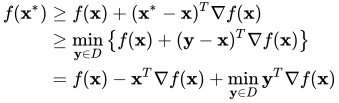
The latter optimization problem is solved in every iteration of the Frank–Wolfe algorithm, therefore the solution of the direction-finding subproblem of the -th iteration can be used to determine increasing lower bounds during each iteration by setting and


Such lower bounds on the unknown optimal value are important in practice because they can be used as a stopping criterion, and give an efficient certificate of the approximation quality in every iteration, since always .

It has been shown that this corresponding duality gap, that is the difference between and the lower bound , decreases with the same convergence rate, i.e.


Notes
[edit]- ^ Levitin, E. S.; Polyak, B. T. (1966). "Constrained minimization methods". USSR Computational Mathematics and Mathematical Physics. 6 (5): 1. doi:10.1016/0041-5553(66)90114-5.
- ^ Frank, M.; Wolfe, P. (1956). "An algorithm for quadratic programming". Naval Research Logistics Quarterly. 3 (1–2): 95–110. doi:10.1002/nav.3800030109.
- ^ Dunn, J. C.; Harshbarger, S. (1978). "Conditional gradient algorithms with open loop step size rules". Journal of Mathematical Analysis and Applications. 62 (2): 432. doi:10.1016/0022-247X(78)90137-3.
- ^ Clarkson, K. L. (2010). "Coresets, sparse greedy approximation, and the Frank-Wolfe algorithm". ACM Transactions on Algorithms. 6 (4): 1–30. CiteSeerX 10.1.1.145.9299. doi:10.1145/1824777.1824783.
- ^ Fukushima, M. (1984). "A modified Frank-Wolfe algorithm for solving the traffic assignment problem". Transportation Research Part B: Methodological. 18 (2): 169–177. doi:10.1016/0191-2615(84)90029-8.
- ^ Bertsekas, Dimitri (1999). Nonlinear Programming. Athena Scientific. p. 215. ISBN 978-1-886529-00-7.
Bibliography
[edit]- Jaggi, Martin (2013). "Revisiting Frank–Wolfe: Projection-Free Sparse Convex Optimization". Journal of Machine Learning Research: Workshop and Conference Proceedings. 28 (1): 427–435. (Overview paper)
- The Frank–Wolfe algorithm description
- Nocedal, Jorge; Wright, Stephen J. (2006). Numerical Optimization (2nd ed.). Berlin, New York: Springer-Verlag. ISBN 978-0-387-30303-1..
External links
[edit]- https://conditional-gradients.org/: a survey of Frank–Wolfe algorithms.
- Marguerite Frank giving a personal account of the history of the algorithm
See also
[edit]
|  | |||||||||||||||||
|
| ||||||||||||||||||
| ||||||||||||||||||
Frank–Wolfe algorithm
View on GrokipediaIntroduction
History
The Frank–Wolfe algorithm was developed in 1956 by mathematicians Marguerite Frank and Philip Wolfe at Princeton University as part of early operations research initiatives.[1] Their work addressed the need for efficient methods to solve constrained optimization problems emerging in post-World War II mathematical modeling for resource allocation and planning.[7] The algorithm was introduced in their seminal paper, "An algorithm for quadratic programming," published in the Naval Research Logistics Quarterly.[1] This publication focused on minimizing quadratic objective functions subject to linear constraints, a formulation prevalent in economic models such as input-output analysis and production planning.[8] The approach built on the convex optimization landscape following George Dantzig's 1947 simplex method for linear programming, extending tools to handle nonlinearity in operations research applications.[9] Early motivations for the algorithm stemmed from quadratic programming challenges in economics, where such problems modeled equilibrium conditions in markets and resource distribution under constraints. Although not explicitly detailed in the original paper, the method's structure lent itself to applications like traffic equilibrium problems, which were formulated as quadratic programs around the same era in works on transportation economics.[10] Independently, a similar method known as the conditional gradient approach appeared in Soviet literature shortly thereafter, developed by E. S. Levitin and B. T. Polyak in their 1966 paper "Constrained minimization methods." This work generalized the technique for broader convex minimization tasks, reflecting parallel advancements in optimization theory during the Cold War era.[11]Overview
The Frank–Wolfe algorithm is a first-order iterative method designed for minimizing smooth convex functions subject to convex constraints, particularly when the feasible set admits efficient linear minimization oracles.[1] Introduced in 1956 by Marguerite Frank and Philip Wolfe, it serves as an alternative to projection-based methods in constrained optimization.[8] A primary advantage of the Frank–Wolfe algorithm lies in its projection-free nature, which eliminates the need for computationally expensive Euclidean projections onto the feasible set, unlike projected gradient descent.[2] This makes it especially suitable for large-scale problems where constraints exhibit structured geometry, such as probability simplices or nuclear norm balls, allowing the use of inexpensive linear optimization subroutines instead.[12] In comparison to other first-order methods, it requires only linear minimization oracles per iteration, which can be significantly cheaper than projections for high-dimensional or complex constraint sets. Intuitively, the algorithm proceeds by iteratively approximating the objective function via linearization at the current point to identify a feasible descent direction, then advancing along a convex combination of the current iterate and this direction.[13] This approach promotes sparsity in solutions and maintains feasibility throughout, enhancing its applicability in modern machine learning tasks like matrix completion and sparse regression.[2]Problem Formulation
Standard Setting
The Frank–Wolfe algorithm targets the convex optimization problem of minimizing a smooth convex objective function $ f: \mathbb{R}^n \to \mathbb{R} $ over a compact convex feasible set $ C \subseteq \mathbb{R}^n $.[14] The problem is formally stated asKey Assumptions
The Frank–Wolfe algorithm is designed for constrained convex optimization problems of the form , where it relies on several key mathematical assumptions to ensure well-defined iterates and convergence guarantees. These conditions pertain to the objective function , the feasible set , and the computational access to optimization subproblems.[16] A fundamental requirement is the convexity of both and . The function must be convex, satisfying for all and ; this ensures that the first-order Taylor approximation lower-bounds , enabling descent directions identified via linear minimization to reduce the objective. Similarly, is a convex set, meaning that for any and , the point also lies in ; convexity of preserves feasibility during convex combinations of iterates. Additionally, is assumed to be compact, which implies it is closed and bounded.[16][3] Smoothness of is another core assumption, requiring the gradient to be Lipschitz continuous with constant . Formally, this means for all , or equivalently, . This -smoothness bounds the approximation error in the linearization step, controlling the curvature and preventing excessive deviation between the true function and its linear model, which is essential for sublinear convergence rates.[16][3] The compactness of further implies a finite diameter , where the supremum is taken with respect to a given norm (often the Euclidean norm). This boundedness ensures that all iterates remain confined within a region of finite size, stabilizing the algorithm's behavior and allowing uniform bounds on duality gaps and progress measures across iterations. Without boundedness, iterates could potentially escape to infinity, undermining convergence.[16] The algorithm also presupposes efficient access to a linear minimization oracle (LMO) over , capable of solving subproblems for any direction vector (typically at the current iterate ). This oracle must be computationally tractable, often leveraging the structure of (e.g., simplices or spectrahedra) to avoid full projections; its efficiency is a hallmark of the method's applicability to high-dimensional or structured constraints.[16][3] Under these assumptions, the algorithm achieves sublinear convergence, but optional stronger conditions can yield improved rates. In particular, if is -strongly convex for some , satisfying for all , then linear convergence is possible, especially when combined with exact line search or adaptive variants. Strong convexity is not required for the basic method but enhances theoretical and practical performance in applications like machine learning.[16]Algorithm Description
Core Steps
The Frank–Wolfe algorithm addresses constrained optimization problems of the form , where is a differentiable convex function and is a compact convex set.[15][2] The procedure begins with the selection of an initial feasible point .[15] In each subsequent iteration , the algorithm computes a search direction by solving , which identifies the point in that minimizes the first-order linear approximation of at the current iterate .[15][2] A step size is then selected, and the iterate is updated via the convex combination , ensuring that remains feasible in by the convexity of the constraint set.[15][2] This update interprets as a promising descent direction derived from the linearized objective, with controlling the extent to which the current point blends toward this direction to reduce the function value while preserving feasibility.[2] The duality gap at iterate is defined as , which upper-bounds the primal optimality gap and serves as a natural stopping criterion.[2] The full procedure is outlined in the following pseudocode, which iterates until the duality gap falls below a tolerance :Require: Initial point x_0 ∈ C, tolerance ε > 0
k ← 0
while g(x_k) ≥ ε do
s_k ← argmin_{s ∈ C} ⟨∇f(x_k), s⟩
γ_k ∈ [0,1] // step size, e.g., via exact or approximate [line search](/page/Line_search)
x_{k+1} ← (1 - γ_k) x_k + γ_k s_k
k ← k + 1
end while
return x_k