Hubbry Logo
SimplexSimplexMain
Open search
Simplex
Community hub
Simplex
logo
8 pages, 0 posts
0 subscribers
Be the first to start a discussion here.
Contribute something
Simplex
Simplex
from Wikipedia
The four simplexes that can be fully represented in 3D space.

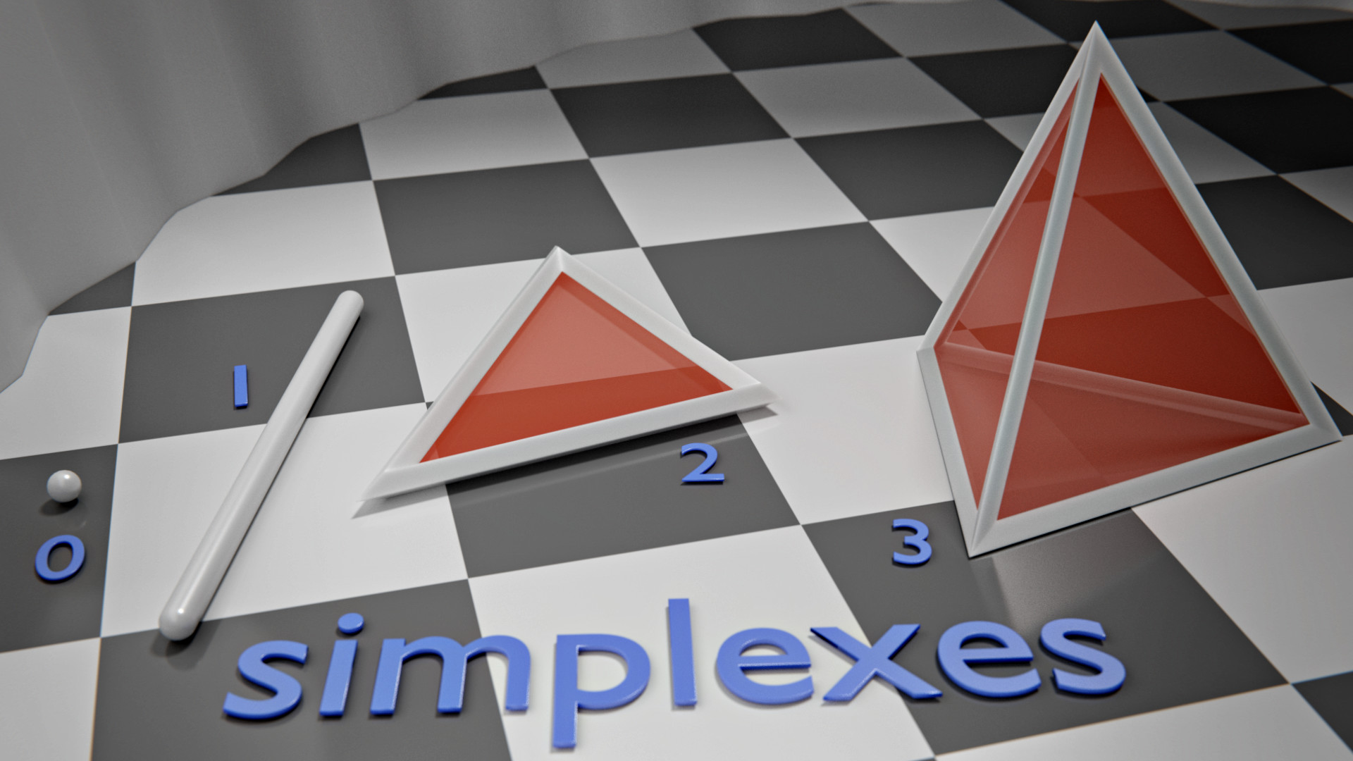
In geometry, a simplex (plural: simplexes or simplices) is a generalization of the notion of a triangle or tetrahedron to arbitrary dimensions. The simplex is so-named because it represents the simplest possible polytope in any given dimension. For example,

Specifically, a k-simplex is a k-dimensional polytope that is the convex hull of its k + 1 vertices. More formally, suppose the k + 1 points are affinely independent, which means that the k vectors are linearly independent. Then, the simplex determined by them is the set of points

A regular simplex[1] is a simplex that is also a regular polytope. A regular k-simplex may be constructed from a regular (k − 1)-simplex by connecting a new vertex to all original vertices by the common edge length.

The standard simplex or probability simplex[2] is the k-dimensional simplex whose vertices are the k + 1 standard unit vectors in or, in other words,

In topology and combinatorics, it is common to "glue together" simplices to form a simplicial complex.

The geometric simplex and simplicial complex should not be confused with the abstract simplicial complex, in which a simplex is simply a finite set and the complex is a family of such sets that is closed under taking subsets.

History

[edit]

The concept of a simplex was known to William Kingdon Clifford, who wrote about these shapes in 1886[clarification needed] but called them "prime confines". Henri Poincaré, writing about algebraic topology in 1900, called them "generalized tetrahedra". In 1902 Pieter Hendrik Schoute described the concept first with the Latin superlative simplicissimum ("simplest") and then with the same Latin adjective in the normal form simplex ("simple").[3][better source needed]

The regular simplex family is the first of three regular polytope families, labeled by Donald Coxeter as αn, the other two being the cross-polytope family, labeled as βn, and the hypercubes, labeled as γn. A fourth family, the tessellation of n-dimensional space by infinitely many hypercubes, he labeled as δn.[4]

Elements

[edit]

The convex hull of any nonempty subset of the n + 1 points that define an n-simplex is called a face of the simplex. Faces are simplices themselves. In particular, the convex hull of a subset of size m + 1 (of the n + 1 defining points) is an m-simplex, called an m-face of the n-simplex. The 0-faces (i.e., the defining points themselves as sets of size 1) are called the vertices (singular: vertex), the 1-faces are called the edges, the (n − 1)-faces are called the facets, and the sole n-face is the whole n-simplex itself. In general, the number of m-faces is equal to the binomial coefficient .[5] Consequently, the number of m-faces of an n-simplex may be found in column (m + 1) of row (n + 1) of Pascal's triangle. A simplex A is a coface of a simplex B if B is a face of A. Face and facet can have different meanings when describing types of simplices in a simplicial complex.

The extended f-vector for an n-simplex can be computed by (1,1)n+1, like the coefficients of polynomial products. For example, a 7-simplex is (1,1)8 = (1,2,1)4 = (1,4,6,4,1)2 = (1,8,28,56,70,56,28,8,1).

The number of 1-faces (edges) of the n-simplex is the n-th triangle number, the number of 2-faces of the n-simplex is the (n − 1)th tetrahedron number, the number of 3-faces of the n-simplex is the (n − 2)th 5-cell number, and so on.

n-Simplex elements[6]
Δn Name Schläfli
Coxeter
0-
faces
(vertices)
1-
faces
(edges)
2-
faces
(faces)
3-
faces
(cells)
4-
faces
 
5-
faces
 
6-
faces
 
7-
faces
 
8-
faces
 
9-
faces
 
10-
faces
 
Sum
= 2n+1 − 1
Δ0 0-simplex
(point)
( )
1                     1
Δ1 1-simplex
(line segment)
{ } = ( ) ∨ ( ) = 2⋅( )
2 1                   3
Δ2 2-simplex
(triangle)
{3} = 3⋅( )
3 3 1                 7
Δ3 3-simplex
(tetrahedron)
{3,3} = 4⋅( )
4 6 4 1               15
Δ4 4-simplex
(5-cell)
{33} = 5⋅( )
5 10 10 5 1             31
Δ5 5-simplex {34} = 6⋅( )
6 15 20 15 6 1           63
Δ6 6-simplex {35} = 7⋅( )
7 21 35 35 21 7 1         127
Δ7 7-simplex {36} = 8⋅( )
8 28 56 70 56 28 8 1       255
Δ8 8-simplex {37} = 9⋅( )
9 36 84 126 126 84 36 9 1     511
Δ9 9-simplex {38} = 10⋅( )
10 45 120 210 252 210 120 45 10 1   1023
Δ10 10-simplex {39} = 11⋅( )
11 55 165 330 462 462 330 165 55 11 1 2047

An n-simplex is the polytope with the fewest vertices that requires n dimensions. Consider a line segment AB as a shape in a 1-dimensional space (the 1-dimensional space is the line in which the segment lies). One can place a new point C somewhere off the line. The new shape, triangle ABC, requires two dimensions; it cannot fit in the original 1-dimensional space. The triangle is the 2-simplex, a simple shape that requires two dimensions. Consider a triangle ABC, a shape in a 2-dimensional space (the plane in which the triangle resides). One can place a new point D somewhere off the plane. The new shape, tetrahedron ABCD, requires three dimensions; it cannot fit in the original 2-dimensional space. The tetrahedron is the 3-simplex, a simple shape that requires three dimensions. Consider tetrahedron ABCD, a shape in a 3-dimensional space (the 3-space in which the tetrahedron lies). One can place a new point E somewhere outside the 3-space. The new shape ABCDE, called a 5-cell, requires four dimensions and is called the 4-simplex; it cannot fit in the original 3-dimensional space. (It also cannot be visualized easily.) This idea can be generalized, that is, adding a single new point outside the currently occupied space, which requires going to the next higher dimension to hold the new shape. This idea can also be worked backward: the line segment we started with is a simple shape that requires a 1-dimensional space to hold it; the line segment is the 1-simplex. The line segment itself was formed by starting with a single point in 0-dimensional space (this initial point is the 0-simplex) and adding a second point, which required the increase to 1-dimensional space.

More formally, an (n + 1)-simplex can be constructed as a join (∨ operator) of an n-simplex and a point, ( ). An (m + n + 1)-simplex can be constructed as a join of an m-simplex and an n-simplex. The two simplices are oriented to be completely normal from each other, with translation in a direction orthogonal to both of them. A 1-simplex is the join of two points: ( ) ∨ ( ) = 2 ⋅ ( ). A general 2-simplex (scalene triangle) is the join of three points: ( ) ∨ ( ) ∨ ( ). An isosceles triangle is the join of a 1-simplex and a point: { } ∨ ( ). An equilateral triangle is 3 ⋅ ( ) or {3}. A general 3-simplex is the join of 4 points: ( ) ∨ ( ) ∨ ( ) ∨ ( ). A 3-simplex with mirror symmetry can be expressed as the join of an edge and two points: { } ∨ ( ) ∨ ( ). A 3-simplex with triangular symmetry can be expressed as the join of an equilateral triangle and 1 point: 3.( )∨( ) or {3}∨( ). A regular tetrahedron is 4 ⋅ ( ) or {3,3} and so on.

The numbers of faces in the above table are the same as in Pascal's triangle, without the left diagonal.
The total number of faces is always a power of two minus one. This figure (a projection of the tesseract) shows the centroids of the 15 faces of the tetrahedron.

In some conventions,[7] the empty set is defined to be a (−1)-simplex. The definition of the simplex above still makes sense if n = −1. This convention is more common in applications to algebraic topology (such as simplicial homology) than to the study of polytopes.

Symmetric graphs of regular simplices

[edit]

These Petrie polygons (skew orthogonal projections) show all the vertices of the regular simplex on a circle, and all vertex pairs connected by edges.


1

2

3

4

5

6

7

8

9

10

11

12

13

14

15

16

17

18

19

20

Standard simplex

[edit]
The standard 2-simplex in R3

The standard n-simplex (or unit n-simplex) is the subset of Rn+1 given by

.

The simplex Δn lies in the affine hyperplane obtained by removing the restriction ti ≥ 0 in the above definition.

The n + 1 vertices of the standard n-simplex are the points eiRn+1, where

e0 = (1, 0, 0, ..., 0),
e1 = (0, 1, 0, ..., 0),
en = (0, 0, 0, ..., 1).

A standard simplex is an example of a 0/1-polytope, with all coordinates as 0 or 1. It can also be seen one facet of a regular (n + 1)-orthoplex.

There is a canonical map from the standard n-simplex to an arbitrary n-simplex with vertices (v0, ..., vn) given by

The coefficients ti are called the barycentric coordinates of a point in the n-simplex. Such a general simplex is often called an affine n-simplex, to emphasize that the canonical map is an affine transformation. It is also sometimes called an oriented affine n-simplex to emphasize that the canonical map may be orientation preserving or reversing.

More generally, there is a canonical map from the standard -simplex (with n vertices) onto any polytope with n vertices, given by the same equation (modifying indexing):

These are known as generalized barycentric coordinates, and express every polytope as the image of a simplex:

A commonly used function from Rn to the interior of the standard -simplex is the softmax function, or normalized exponential function; this generalizes the standard logistic function.

Examples

[edit]
  • Δ0 is the point 1 in R1.
  • Δ1 is the line segment joining (1, 0) and (0, 1) in R2.
  • Δ2 is the equilateral triangle with vertices (1, 0, 0), (0, 1, 0) and (0, 0, 1) in R3.
  • Δ3 is the regular tetrahedron with vertices (1, 0, 0, 0), (0, 1, 0, 0), (0, 0, 1, 0) and (0, 0, 0, 1) in R4.
  • Δ4 is the regular 5-cell with vertices (1, 0, 0, 0, 0), (0, 1, 0, 0, 0), (0, 0, 1, 0, 0), (0, 0, 0, 1, 0) and (0, 0, 0, 0, 1) in R5.

Increasing coordinates

[edit]

An alternative coordinate system is given by taking the indefinite sum:

This yields the alternative presentation by order, namely as nondecreasing n-tuples between 0 and 1:

Geometrically, this is an n-dimensional subset of (maximal dimension, codimension 0) rather than of (codimension 1). The facets, which on the standard simplex correspond to one coordinate vanishing, here correspond to successive coordinates being equal, while the interior corresponds to the inequalities becoming strict (increasing sequences).

A key distinction between these presentations is the behavior under permuting coordinates – the standard simplex is stabilized by permuting coordinates, while permuting elements of the "ordered simplex" do not leave it invariant, as permuting an ordered sequence generally makes it unordered. Indeed, the ordered simplex is a (closed) fundamental domain for the action of the symmetric group on the n-cube, meaning that the orbit of the ordered simplex under the n! elements of the symmetric group divides the n-cube into mostly disjoint simplices (disjoint except for boundaries), showing that this simplex has volume 1/n!. Alternatively, the volume can be computed by an iterated integral, whose successive integrands are 1, x, x2/2, x3/3!, ..., xn/n!.

A further property of this presentation is that it uses the order but not addition, and thus can be defined in any dimension over any ordered set, and for example can be used to define an infinite-dimensional simplex without issues of convergence of sums.

Projection onto the standard simplex

[edit]

Especially in numerical applications of probability theory, a projection onto the standard simplex is of interest. Given , possibly with coordinates that are negative or in excess of 1, the closest point  on the simplex has coordinates

where  is chosen such that 

can be easily calculated from sorting the coordinates of .[8] The sorting approach takes  complexity, which can be improved to O(n) complexity via median-finding algorithms.[9] Projecting onto the simplex is computationally similar to projecting onto the ball. Also see Integer programming.

Corner of cube

[edit]

Finally, a simple variant is to replace "summing to 1" with "summing to at most 1"; this raises the dimension by 1, so to simplify notation, the indexing changes:

This yields an n-simplex as a corner of the n-cube, and is a standard orthogonal simplex. This is the simplex used in the simplex method, which is based at the origin, and locally models a vertex on a polytope with n facets.

Cartesian coordinates for a regular n-dimensional simplex in Rn

[edit]

One way to write down a regular n-simplex in Rn is to choose two points to be the first two vertices, choose a third point to make an equilateral triangle, choose a fourth point to make a regular tetrahedron, and so on. Each step requires satisfying equations that ensure that each newly chosen vertex, together with the previously chosen vertices, forms a regular simplex. There are several sets of equations that can be written down and used for this purpose. These include the equality of all the distances between vertices; the equality of all the distances from vertices to the center of the simplex; the fact that the angle subtended through the new vertex by any two previously chosen vertices is ; and the fact that the angle subtended through the center of the simplex by any two vertices is .

It is also possible to directly write down a particular regular n-simplex in Rn which can then be translated, rotated, and scaled as desired. One way to do this is as follows. Denote the basis vectors of Rn by e1 through en. Begin with the standard (n − 1)-simplex which is the convex hull of the basis vectors. By adding an additional vertex, these become a face of a regular n-simplex. The additional vertex must lie on the line perpendicular to the barycenter of the standard simplex, so it has the form (α/n, ..., α/n) for some real number α. Since the squared distance between two basis vectors is 2, in order for the additional vertex to form a regular n-simplex, the squared distance between it and any of the basis vectors must also be 2. This yields a quadratic equation for α. Solving this equation shows that there are two choices for the additional vertex:

Either of these, together with the standard basis vectors, yields a regular n-simplex.

The above regular n-simplex is not centered on the origin. It can be translated to the origin by subtracting the mean of its vertices. By rescaling, it can be given unit side length. This results in the simplex whose vertices are:

for , and

Note that there are two sets of vertices described here. One set uses in each calculation. The other set uses in each calculation.

This simplex is inscribed in a hypersphere of radius .

A different rescaling produces a simplex that is inscribed in a unit hypersphere. When this is done, its vertices are

where , and

The side length of this simplex is .

A highly symmetric way to construct a regular n-simplex is to use a representation of the cyclic group Zn+1 by orthogonal matrices. This is an n × n orthogonal matrix Q such that Qn+1 = I is the identity matrix, but no lower power of Q is. Applying powers of this matrix to an appropriate vector v will produce the vertices of a regular n-simplex. To carry this out, first observe that for any orthogonal matrix Q, there is a choice of basis in which Q is a block diagonal matrix

where each Qi is orthogonal and either 2 × 2 or 1 × 1. In order for Q to have order n + 1, all of these matrices must have order dividing n + 1. Therefore each Qi is either a 1 × 1 matrix whose only entry is 1 or, if n is odd, −1; or it is a 2 × 2 matrix of the form

where each ωi is an integer between zero and n inclusive. A sufficient condition for the orbit of a point to be a regular simplex is that the matrices Qi form a basis for the non-trivial irreducible real representations of Zn+1, and the vector being rotated is not stabilized by any of them.

In practical terms, for n even this means that every matrix Qi is 2 × 2, there is an equality of sets

and, for every Qi, the entries of v upon which Qi acts are not both zero. For example, when n = 4, one possible matrix is

Applying this to the vector (1, 0, 1, 0) results in the simplex whose vertices are

each of which has distance √5 from the others. When n is odd, the condition means that exactly one of the diagonal blocks is 1 × 1, equal to −1, and acts upon a non-zero entry of v; while the remaining diagonal blocks, say Q1, ..., Q(n − 1) / 2, are 2 × 2, there is an equality of sets

and each diagonal block acts upon a pair of entries of v which are not both zero. So, for example, when n = 3, the matrix can be

For the vector (1, 0, 1/2), the resulting simplex has vertices

each of which has distance 2 from the others.

Geometric properties

[edit]

Volume

[edit]

The volume of an n-simplex in n-dimensional space with vertices (v0, ..., vn) is

where each column of the n × n determinant is a vector that points from vertex v0 to another vertex vk.[10] This formula is particularly useful when is the origin.

The expression

employs a Gram determinant and works even when the n-simplex's vertices are in a Euclidean space with more than n dimensions, e.g., a triangle in .

A more symmetric way to compute the volume of an n-simplex in is

Another common way of computing the volume of the simplex is via the Cayley–Menger determinant, which works even when the n-simplex's vertices are in a Euclidean space with more than n dimensions.[11]

Without the 1/n! it is the formula for the volume of an n-parallelotope. This can be understood as follows: Assume that P is an n-parallelotope constructed on a basis of . Given a permutation of , call a list of vertices a n-path if

(so there are n! n-paths and does not depend on the permutation). The following assertions hold:

If P is the unit n-hypercube, then the union of the n-simplexes formed by the convex hull of each n-path is P, and these simplexes are congruent and pairwise non-overlapping.[12] In particular, the volume of such a simplex is

If P is a general parallelotope, the same assertions hold except that it is no longer true, in dimension > 2, that the simplexes need to be pairwise congruent; yet their volumes remain equal, because the n-parallelotope is the image of the unit n-hypercube by the linear isomorphism that sends the canonical basis of to . As previously, this implies that the volume of a simplex coming from a n-path is:

Conversely, given an n-simplex of , it can be supposed that the vectors form a basis of . Considering the parallelotope constructed from and , one sees that the previous formula is valid for every simplex.

Finally, the formula at the beginning of this section is obtained by observing that

From this formula, it follows immediately that the volume under a standard n-simplex (i.e. between the origin and the simplex in Rn+1) is

The volume of a regular n-simplex with unit side length is

as can be seen by multiplying the previous formula by xn+1, to get the volume under the n-simplex as a function of its vertex distance x from the origin, differentiating with respect to x, at   (where the n-simplex side length is 1), and normalizing by the length of the increment, , along the normal vector.

Dihedral angles of the regular n-simplex

[edit]

Any two (n − 1)-dimensional faces of a regular n-dimensional simplex are themselves regular (n − 1)-dimensional simplices, and they have the same dihedral angle of cos−1(1/n).[13][14]

This can be seen by noting that the center of the standard simplex is , and the centers of its faces are coordinate permutations of . Then, by symmetry, the vector pointing from to is perpendicular to the faces. So the vectors normal to the faces are permutations of , from which the dihedral angles are calculated.

Simplices with an "orthogonal corner"

[edit]

An "orthogonal corner" means here that there is a vertex at which all adjacent edges are pairwise orthogonal. It immediately follows that all adjacent faces are pairwise orthogonal. Such simplices are generalizations of right triangles and for them there exists an n-dimensional version of the Pythagorean theorem: The sum of the squared (n − 1)-dimensional volumes of the facets adjacent to the orthogonal corner equals the squared (n − 1)-dimensional volume of the facet opposite of the orthogonal corner.

where are facets being pairwise orthogonal to each other but not orthogonal to , which is the facet opposite the orthogonal corner.[15]

For a 2-simplex, the theorem is the Pythagorean theorem for triangles with a right angle and for a 3-simplex it is de Gua's theorem for a tetrahedron with an orthogonal corner.

Relation to the (n + 1)-hypercube

[edit]

The Hasse diagram of the face lattice of an n-simplex is isomorphic to the graph of the (n + 1)-hypercube's edges, with the hypercube's vertices mapping to each of the n-simplex's elements, including the entire simplex and the null polytope as the extreme points of the lattice (mapped to two opposite vertices on the hypercube). This fact may be used to efficiently enumerate the simplex's face lattice, since more general face lattice enumeration algorithms are more computationally expensive.

The n-simplex is also the vertex figure of the (n + 1)-hypercube. It is also the facet of the (n + 1)-orthoplex.

Topology

[edit]

Topologically, an n-simplex is equivalent to an n-ball. Every n-simplex is an n-dimensional manifold with corners.

Probability

[edit]

In probability theory, the points of the standard n-simplex in (n + 1)-space form the space of possible probability distributions on a finite set consisting of n + 1 possible outcomes. The correspondence is as follows: For each distribution described as an ordered (n + 1)-tuple of probabilities whose sum is (necessarily) 1, we associate the point of the simplex whose barycentric coordinates are precisely those probabilities. That is, the kth vertex of the simplex is assigned to have the kth probability of the (n + 1)-tuple as its barycentric coefficient. This correspondence is an affine homeomorphism.

Aitchison geometry

[edit]

Aitchinson geometry is a natural way to construct an inner product space from the standard simplex . It defines the following operations on simplices and real numbers:

Perturbation (addition)
Powering (scalar multiplication)
Inner product

Compounds

[edit]

Since all simplices are self-dual, they can form a series of compounds;

Algebraic topology

[edit]

In algebraic topology, simplices are used as building blocks to construct an interesting class of topological spaces called simplicial complexes. These spaces are built from simplices glued together in a combinatorial fashion. Simplicial complexes are used to define a certain kind of homology called simplicial homology.

A finite set of k-simplexes embedded in an open subset of Rn is called an affine k-chain. The simplexes in a chain need not be unique; they may occur with multiplicity. Rather than using standard set notation to denote an affine chain, it is instead the standard practice to use plus signs to separate each member in the set. If some of the simplexes have the opposite orientation, these are prefixed by a minus sign. If some of the simplexes occur in the set more than once, these are prefixed with an integer count. Thus, an affine chain takes the symbolic form of a sum with integer coefficients.

Note that each facet of an n-simplex is an affine (n − 1)-simplex, and thus the boundary of an n-simplex is an affine (n − 1)-chain. Thus, if we denote one positively oriented affine simplex as

with the denoting the vertices, then the boundary of σ is the chain

It follows from this expression, and the linearity of the boundary operator, that the boundary of the boundary of a simplex is zero:

Likewise, the boundary of the boundary of a chain is zero: .

More generally, a simplex (and a chain) can be embedded into a manifold by means of smooth, differentiable map . In this case, both the summation convention for denoting the set, and the boundary operation commute with the embedding. That is,

where the are the integers denoting orientation and multiplicity. For the boundary operator , one has:

where ρ is a chain. The boundary operation commutes with the mapping because, in the end, the chain is defined as a set and little more, and the set operation always commutes with the map operation (by definition of a map).

A continuous map to a topological space X is frequently referred to as a singular n-simplex. (A map is generally called "singular" if it fails to have some desirable property such as continuity and, in this case, the term is meant to reflect to the fact that the continuous map need not be an embedding.)[16]

Algebraic geometry

[edit]

Since classical algebraic geometry allows one to talk about polynomial equations but not inequalities, the algebraic standard n-simplex is commonly defined as the subset of affine (n + 1)-dimensional space, where all coordinates sum up to 1 (thus leaving out the inequality part). The algebraic description of this set is which equals the scheme-theoretic description with the ring of regular functions on the algebraic n-simplex (for any ring ).

By using the same definitions as for the classical n-simplex, the n-simplices for different dimensions n assemble into one simplicial object, while the rings assemble into one cosimplicial object (in the category of schemes resp. rings, since the face and degeneracy maps are all polynomial).

The algebraic n-simplices are used in higher K-theory and in the definition of higher Chow groups.

Applications

[edit]

See also

[edit]

Notes

[edit]

References

[edit]
Revisions and contributorsEdit on WikipediaRead on Wikipedia
from Grokipedia
A simplex is a fundamental geometric object in , defined as the of a of n+1 affinely independent points in n-dimensional , generalizing familiar shapes such as , , and to higher dimensions.
  • In zero dimensions, a 0-simplex is simply a point;
  • a 1-simplex is a connecting two points;
  • a 2-simplex forms a with three vertices;
  • a 3-simplex is a bounded by four triangular faces.
These low-dimensional cases illustrate the simplex's role as the simplest in each dimension, possessing the minimal number of vertices and facets required to span the space without redundancy. Analogously to how 2D polygons can be decomposed into triangles, any higher-dimensional polytope can be decomposed into simplices, which can be helpful in some settings like calculations of volume. Beyond pure geometry, simplices form the basic building blocks of simplicial complexes, finite collections of simplices glued together along shared faces to approximate manifolds and other topological objects without self-intersections. Simplices exhibit key properties that make them central to , including the fact that any simplex is itself convex and that its faces—subsimplices formed by subsets of its vertices—fully describe its boundary structure. Moreover, simplices are contractible topological spaces, meaning they can be continuously deformed to a point, which underpins their use in defining for studying the shape of more complex spaces. In optimization, the term "simplex" inspired the naming of the for , developed by in 1947, which efficiently navigates the vertices of polyhedral feasible regions—though the method itself operates on coordinate representations rather than explicit simplices.

Fundamentals

Definition

A simplex is the generalization of a point (0-dimensional), (1-dimensional), (2-dimensional), or (3-dimensional) to arbitrary dimensions, serving as the n-dimensional analogue of these basic geometric figures. Geometrically, an n-simplex is defined as the of n+1 affinely independent points in n-dimensional . Formally, if v0,v1,,vnRnv_0, v_1, \dots, v_n \in \mathbb{R}^n are affinely independent, the n-simplex σ\sigma is given by σ=conv{v0,v1,,vn},\sigma = \mathrm{conv}\{v_0, v_1, \dots, v_n\}, where conv\mathrm{conv} denotes the set of all convex combinations of these points. Points v0,v1,,vnv_0, v_1, \dots, v_n are affinely independent if the vectors v1v0,v2v0,,vnv0v_1 - v_0, v_2 - v_0, \dots, v_n - v_0 are linearly independent in Rn\mathbb{R}^n. For example, in 2-dimensional , three points are affinely independent if they are not collinear, ensuring the forms a with positive area. In 3-dimensional , four points are affinely independent if they are not coplanar, yielding a with positive volume. In general, Rn\mathbb{R}^n admits at most n+1 affinely independent points, which determines the maximum of a simplex in that space. Combinatorially, an n-simplex is specified by a set of n+1 vertices, with all its faces (including itself and the empty set) corresponding to the convex hulls of subsets of these vertices; any subset of the vertices is itself affinely independent, ensuring a hierarchical structure of lower-dimensional simplices. As a convex polytope, the simplex is the simplest such object in n dimensions, requiring exactly n+1 vertices to span the full dimensionality, in contrast to more complex polytopes with additional vertices and facets.

Elements

A simplex in nn-dimensional space is defined by its vertices, which are n+1n+1 affinely independent points that serve as the extreme points spanning the entire structure. These vertices form the 0-dimensional faces, or 0-simplices, and every point within the simplex can be expressed as a of them. The edges of an nn-simplex are its 1-dimensional faces, each connecting a pair of vertices and thus forming line segments between them. The total number of such edges is given by the (n+12)\binom{n+1}{2}, reflecting the combinatorial selection of two vertices from the n+1n+1 available. In general, the kk-faces of an nn-simplex, for 0kn0 \leq k \leq n, are the kk-dimensional sub-simplices generated by any k+1k+1 of the vertices, provided they remain affinely independent. These kk-faces inherit the simplex structure, with their own vertices, edges, and lower-dimensional components scaled down accordingly. The complete enumeration of kk-faces in an nn-simplex yields (n+1k+1)\binom{n+1}{k+1} such elements, capturing the pure combinatorial skeleton of the simplex. The facets represent the highest-dimensional proper faces, specifically the (n1)(n-1)-faces that bound the nn-simplex, each omitting exactly one vertex from the full set. An nn-simplex possesses exactly n+1n+1 facets, one corresponding to each vertex exclusion, forming the immediate boundary layers. The boundary of an nn-simplex is the union of all its proper faces—those of dimension less than nn—excluding the interior points that lie strictly within the convex hull. This boundary structure ensures the simplex is a closed manifold with boundary, topologically equivalent to the (n1)(n-1)-sphere in its facial complex.

Low-Dimensional Examples

A 0-simplex is the simplest geometric object, consisting of a single point with no , serving as the basic building block for higher-dimensional simplices. In one , the 1-simplex takes the form of a defined by two vertices connected by one edge, representing the of these two affinely independent points. The 2-simplex extends this to a filled in the plane, comprising three vertices, three edges forming its boundary, and three degenerate 0-dimensional faces at the vertices themselves, with the entire enclosing a 2-dimensional area. To visualize, consider points A, B, and C forming the corners, where AB, BC, and CA are the edges. A 3-simplex is a in , featuring four vertices, six edges connecting them pairwise, four triangular 2-simplex faces, with the itself as the 3-simplex. For intuition, imagine vertices at the corners of a with a triangular base, where each face is a triangle and all edges meet at the vertices. Simplices need not be regular or symmetric; for instance, an oblique with unequal side lengths and angles exemplifies a non-regular 2-simplex, while an irregular with varying edge lengths and face shapes demonstrates the generality in three dimensions.

History

Origins

The concept of the simplex traces its origins to , where the emerged as the fundamental building block for plane figures. In 's Elements, composed around 300 BCE, triangles are treated as the basic trilateral figures, serving as the basis for propositions on congruence, similarity, and area throughout the foundational text of . This treatment established the triangle as the simplest , embodying the core principles of and that would later generalize to higher dimensions. The revival and formalization of the simplex concept occurred in the amid advances in synthetic and . Jakob Steiner played a pivotal role in the through his work on polyhedral theory, recognizing the minimal generated by n+1 affinely independent points in n-dimensional space as the foundational element within his systematic exploration of geometric dependencies. Steiner's approach emphasized this primitive's role as the generator of more complex polytopes, providing a synthetic framework for understanding dimensional dependencies without coordinates. Arthur Cayley further advanced this idea during the 1840s and 1850s, integrating analytical methods into higher-dimensional and extending Steiner's polyhedral insights to n dimensions. Cayley's papers on the geometry of position and multi-dimensional forms treated these minimal polytopes (later termed simplices) as essential primitives for coordinate-free descriptions, bridging synthetic and algebraic perspectives. The term "simplex" for these minimal polytopes was introduced by Dutch mathematician Pieter Hendrik Schoute in his early 20th-century work on multidimensional geometry, around 1902–1905. A defining milestone arrived in 1872 with Felix Klein's , which classified geometries by their underlying transformation groups and positioned the minimal as the canonical figure in . Klein's framework highlighted its invariance under affine transformations, solidifying its status as the foundational convex body for affine structures and distinguishing it from Euclidean or projective counterparts.

Modern Developments

In the early , advanced the understanding of simplices through his development of simplicial complexes in . In his 1922 work Analysis Situs, Veblen developed a combinatorial framework for manifolds using simplicial decompositions, establishing the homology of simplicial complexes as a topological invariant, which laid foundational groundwork for modern . Building on these ideas, made significant contributions to applications of simplices during the 1930s to 1950s. Cartan's seminars and collaborations, particularly his 1956 co-authored book with , generalized to chain complexes over arbitrary rings, enabling broader applications in sheaf theory and that influenced subsequent topological developments. In the mid-20th century, simplices gained prominence in optimization through George Dantzig's 1947 invention of the for . This method iteratively traverses vertices of the feasible region's polyhedral representation—often a simplex or union of simplices—to solve linear optimization problems efficiently, revolutionizing and economic modeling despite its theoretical worst-case exponential . The late 20th century saw simplices applied to statistical analysis of by John Aitchison in the 1980s. Aitchison's 1982 paper introduced the simplex as a for proportions summing to unity, developing a log-ratio on the simplex to handle constraints in , such as geochemical compositions, which overcame issues with Euclidean metrics and spurred the field of compositional data analysis. Post-2000 advancements in have enhanced simplex-based algorithms, particularly in Delaunay triangulations, which decompose point sets into simplices maximizing minimum angles for in finite element methods. Reviews highlight progress in parallel and GPU-accelerated implementations, such as randomized incremental constructions achieving near-optimal for large-scale 3D triangulations, improving simulations in and . In the 2020s, high-dimensional simplices have emerged in for modeling data manifolds via topological deep learning. Frameworks like simplicial neural networks extend graph convolutions to higher-order interactions on simplicial complexes, capturing multi-way relationships in datasets such as social networks or molecular structures; for instance, HiPoNet (2025) enables end-to-end learning on high-dimensional simplicial inputs for tasks like , demonstrating improved performance on benchmarks over traditional manifold methods.

Representations

Standard Simplex

The standard nn-simplex, denoted Δn\Delta^n, is the defined as Δn={(x0,,xn)Rn+1  |  xi0    i,i=0nxi=1}.\Delta^n = \left\{ (x_0, \dots, x_n) \in \mathbb{R}^{n+1} \;\middle|\; x_i \geq 0 \;\forall\; i, \sum_{i=0}^n x_i = 1 \right\}.
Add your contribution
Related Hubs
Contribute something
User Avatar
No comments yet.