Hertzsprung–Russell diagram

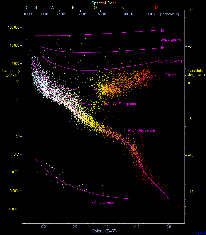
The Hertzsprung–Russell diagram (HR diagram or H–R diagram) is a fundamental astronomical tool that plots stars' luminosity (or absolute magnitude) against their surface temperature (or spectral type), revealing key patterns in stellar properties and evolution.^[1] It was independently developed in 1912 by Danish astronomer Ejnar Hertzsprung and American astronomer Henry Norris Russell, using observational data to compare stars' brightness and color.^[2] The diagram's horizontal axis typically runs from hot, blue stars (spectral types O and B, around 30,000–50,000 K) on the left to cool, red stars (types K and M, around 3,000–4,000 K) on the right, while the vertical axis increases upward from low luminosity (dimmer stars) to high luminosity (brighter stars).^[3] Approximately 90% of stars cluster along a diagonal band known as the main sequence, where stars like the Sun spend most of their hydrogen-fusing lifetimes, with position determined primarily by mass—hotter, more massive stars at the upper left evolve faster, while cooler, less massive ones at the lower right last longer.^[1] Above the main sequence lie the red giants and supergiants, representing later evolutionary stages where stars expand and brighten after exhausting core hydrogen, and below it are the faint white dwarfs, the remnants of low- to medium-mass stars that have shed their outer layers.^[3] This scatter plot not only classifies stars by intrinsic properties but also serves as a cornerstone for understanding stellar life cycles, as it captures snapshots of stars at different ages and masses, enabling predictions about evolution, composition, and even distances via standard candles like Cepheid variables in the instability strip.^[1] Developed from early 20th-century spectroscopic data, including classifications by Annie Jump Cannon, the HR diagram remains essential for modern astrophysics, from cluster analysis to galaxy formation studies.^[3]

Historical Development

Origins and Independent Work

Ejnar Hertzsprung, a Danish astronomer, began his investigations into stellar luminosities in 1905 with a study focused on the absolute magnitudes of stars in the Pleiades and Hyades open clusters.^[4] In this work, published as "Zur Strahlung der Sterne" in the Zeitschrift für wissenschaftliche Photographie, Hertzsprung plotted apparent magnitudes against spectral types derived from photographic spectra, revealing distinct patterns in stellar brightness for stars of similar colors. Building on the spectral classifications of Antonia Maury, which showed irregularities in brightness for same-type stars, his analysis identified two types of red stars: small, faint dwarfs and large, bright giants.^[4][5] His primary motivation was to improve distance determinations to these clusters by identifying reliable luminosity indicators, leveraging the assumption that stars within a cluster share a common distance and thus exhibit a consistent sequence in magnitude-spectral type space for main sequence fitting.^[6] In 1908, Hertzsprung created an early version of the diagram for the Pleiades cluster in his notebook, analyzing field stars and cluster members more broadly, but this work remained unpublished at the time.^[7] These findings stemmed from his ongoing interest in spectroscopic data to refine cluster distances, as patterns in the plots allowed calibration against known nearby stars like the Sun.^[7] Independently, American astronomer Henry Norris Russell developed a similar framework in 1913, motivated by advances in measuring trigonometric parallaxes and refining stellar classification systems.^[8] At a meeting of the American Astronomical Society in December 1913, Russell presented a diagram plotting absolute luminosity against spectral type for approximately 300 field stars, uncovering analogous groupings of bright giants and faint dwarfs, as well as a dominant sequence of intermediate-luminosity stars.^[9] His work emphasized spectroscopic parallaxes—estimating distances from spectral features correlated with luminosity—to enhance understanding of stellar populations and evolution.^[10] The geographical separation between Hertzsprung in Denmark and Russell in the United States prevented early collaboration, leading to parallel discoveries without direct influence until later exchanges.^[11]

Early Publications and Adoption

Ejnar Hertzsprung's pioneering observations on the relationship between stellar colors and luminosities appeared in his 1905 paper "Zur Strahlung der Sterne," published in the obscure Zeitschrift für wissenschaftliche Photographie, Photophysik und Photochemie, which received limited circulation among astronomers. Independently, Henry Norris Russell constructed a comparable diagram in 1913, using available parallax data to plot absolute magnitudes against spectral types; this was first presented at the American Astronomical Society meeting in December 1913 and formally published in 1914 as "Relations Between the Spectra and Other Characteristics of the Stars" in Popular Astronomy.^[9][8] Hertzsprung advanced the conceptual framework in 1911 with his paper in Publikationen des Astrophysikalischen Observatoriums zu Potsdam, where he published the first diagrams and formalized the terms "Zwergsterne" (dwarf stars) for the fainter sequence and "Riesensterne" (giant stars) for the brighter one among red stars, emphasizing their distinct luminosities despite similar spectra.^[12] Russell built on this distinction in his 1914 publication, refining the diagram by explicitly using absolute magnitude on the vertical axis—calculated from apparent magnitudes and trigonometric parallaxes—against Harvard spectral classes on the horizontal axis, thereby clarifying the separation between dwarfs and giants across a broader stellar sample.^[9] The diagram's adoption gained momentum following Russell's 1913 presentation to the American Astronomical Society, where it was recognized as a tool for classifying stellar properties beyond apparent brightness.^[8] A key milestone came in 1925 with Cecilia Payne-Gaposchkin's PhD thesis Stellar Atmospheres at Harvard, where she integrated the diagram to correlate spectral lines with surface temperatures, demonstrating that stars across the plot share similar compositions dominated by hydrogen and helium, thus linking observational data to physical interpretations of luminosity and spectra.^[13] Early acceptance faced significant hurdles due to sparse and imprecise measurements of stellar distances and luminosities in the pre-1920s era, as deriving absolute magnitudes required reliable trigonometric parallaxes, which were available for only a few nearby stars.^[14] These limitations were largely overcome by Harlow Shapley's investigations of globular clusters starting in the mid-1910s, particularly his 1918 analysis using the period-luminosity relation of RR Lyrae variables to establish distances to over 60 clusters, allowing construction of reliable color-magnitude diagrams for cluster stars at uniform distances and populating the plot with thousands of data points. Although Hertzsprung and Russell worked independently without collaboration, the diagram received its first joint attribution as the "Hertzsprung-Russell diagram" in astronomical literature during the 1940s, coinciding with advances in stellar evolution theory that solidified its foundational role.^[14]

Fundamental Concepts

Plotted Stellar Parameters

The Hertzsprung–Russell (HR) diagram plots stars based on two primary parameters: luminosity (L), which measures the total energy output of a star across all wavelengths, and effective temperature (T_eff), which approximates the temperature of the star's photosphere assuming blackbody radiation. Luminosity quantifies the intrinsic brightness of a star, typically expressed in solar units (L_⊙), and serves as the vertical axis to reveal evolutionary stages and physical properties. Effective temperature, in kelvin (K), is determined by fitting the observed spectral energy distribution to a blackbody curve or using color indices such as B-V, providing insight into the star's surface conditions and atmospheric composition. These parameters allow astronomers to map stellar populations without direct measurement of every star's radius or internal structure. Luminosity is derived from the star's observed flux F (energy received per unit area per unit time) and its distance d via the inverse-square law: $L = 4\pi d^2 F$L=4πd2F. Flux is measured through photometry, while distances require independent methods to convert apparent brightness into absolute values. Effective temperature is inferred from the peak wavelength of the star's spectrum using Wien's displacement law or by comparing broadband colors to theoretical models, as real stellar spectra deviate slightly from ideal blackbodies due to absorption lines. These derivations assume isotropic emission and spherical symmetry, foundational to plotting reliable HR diagrams. The spectral classification system, refined by Annie Jump Cannon in the early 20th century, correlates directly with T_eff through the OBAFGKM sequence, where earlier types indicate hotter stars. O-type stars exceed 30,000 K, characterized by ionized helium lines, while M-type stars fall below 3,500 K, showing strong molecular bands; the Sun, a G-type star, has T_eff ≈ 5,800 K. This Harvard classification, based on spectroscopic features, provides a practical proxy for temperature without full spectral fitting. To plot luminosity accurately, absolute bolometric magnitude (M_{\rm bol}) often serves as a logarithmic proxy, related by $M_{\rm bol} = -2.5 \log_{10}(L / L_\odot) + 4.74$Mbol​=−2.5log10​(L/L⊙​)+4.74^[15], where the constant is the solar bolometric magnitude. In observational contexts, absolute visual magnitude (M_v) is frequently used instead, related to bolometric magnitude via bolometric corrections (BC): $M_{\rm bol} = M_v + {\rm BC}(T_{\rm eff})$Mbol​=Mv​+BC(Teff​), which can reach -3 magnitudes for hot O stars due to ultraviolet excess. These corrections, calibrated from model atmospheres, ensure the plotted values reflect total energy output. Apparent magnitude alone is insufficient for HR diagram construction, as it conflates luminosity with distance; absolute values demand trigonometric parallaxes from missions like Hipparcos or Gaia, measuring angular shifts against background stars, or cluster methods assuming coeval distances for member stars. Parallaxes yield precise d up to several kiloparsecs, enabling L calibration for nearby samples, while cluster fitting extends this to farther groups by aligning their main sequences to known standards.

Axes and Scaling Conventions

The standard Hertzsprung–Russell (HR) diagram employs a vertical axis representing stellar luminosity in logarithmic units, typically expressed as $\log (L / L_\odot)$log(L/L⊙​), where $L$L is the star's luminosity and $L_\odot$L⊙​ is the Sun's luminosity (approximately $3.828 \times 10^{26}$3.828×1026 W), increasing upward from values around $-4$−4 to $6$. The horizontal axis plots [effective temperature](/page/Effective_temperature)$.Thehorizontalaxisplots[effectivetemperature](/page/Effectivet​emperature)T_{\rm eff}$on a [logarithmic scale](/page/Logarithmic_scale) as$ona[logarithmicscale](/page/Logarithmics​cale)as\log T_{\rm eff}, ranging from about $3.5 (corresponding to roughly 3,000 K for cool stars) to $4.7$ (about 50,000 K for hot stars), with the scale decreasing from left to right to reflect hotter stars on the left and cooler ones on the right. This configuration allows for a clear visualization of the empirical relations between stellar brightness and temperature, as originally conceptualized in early 20th-century plots but refined in modern theoretical forms. Logarithmic scaling for both axes is essential due to the enormous dynamic range in stellar properties: luminosities span over 10 orders of magnitude from faint white dwarfs at $10^{-4} L_\odot$10−4L⊙​ to luminous supergiants exceeding $10^6 L_\odot$106L⊙​, while effective temperatures vary by factors of up to 20 across main-sequence stars. Linear scales would compress the majority of stars—particularly the abundant, lower-luminosity main-sequence population—into a narrow band, obscuring patterns and making the diagram impractical for analysis. This choice aligns with the physical realities of stellar structure, where luminosity $L \propto R^2 T_{\rm eff}^4$L∝R2Teff4​ (from the Stefan–Boltzmann law) naturally leads to logarithmic distributions when plotting diverse stellar types. In observational variants of the HR diagram, the horizontal axis is often replaced by spectral type (O through M, with O hottest on the left), as pioneered by Ejnar Hertzsprung in 1905 and Henry Norris Russell in 1913, who plotted absolute magnitude against spectral class to reveal luminosity gaps. Photometric surveys frequently use color indices such as $B-V$B−V (blue minus visual magnitude) instead, where negative values indicate hot, blue stars and positive values cooler, red ones; this correlates well with $\log T_{\rm eff}$logTeff​ via empirical calibrations. The reversed temperature (or spectral type) axis stems from early 20th-century conventions in stellar spectroscopy, where sequences were ordered from hot (O-type, left) to cool (M-type, right) to match wavelength progression in spectra, a tradition retained for consistency despite the unconventional decreasing scale. Luminosity is commonly converted to absolute bolometric magnitude $M_{\rm bol}$Mbol​ for plotting, using the relation $$M_{\rm bol} = -2.5 \log \left( \frac{L}{L_\odot} \right) + 4.74,$$Mbol​=−2.5log(L⊙​L​)+4.74, where the zero-point $4.74$is set by the [International Astronomical Union](/page/International_Astronomical_Union) such that the Sun has$issetbythe[InternationalAstronomicalUnion](/page/InternationalA​stronomicalU​nion)suchthattheSunhasM_{\rm bol,\odot} = 4.74$at$atL = L_\odot$. Some HR diagram variants incorporate auxiliary axes or overlays, such as lines of constant radius (derived from$.SomeHRdiagramvariantsincorporateauxiliaryaxesoroverlays,suchaslinesofconstantradius(derivedfromL \propto R^2 T_{\rm eff}^4$) or surface gravity$)orsurfacegravity\log g$, to provide additional context on stellar size and density without altering the primary axes.

Diagram Variants

Observational Forms

Observational forms of the Hertzsprung–Russell (HR) diagram rely on empirical data from stellar photometry and astrometry to plot stars' positions based on measured properties. These diagrams typically use color indices, such as B-V, as proxies for effective temperature on the horizontal axis and apparent or absolute visual magnitude (V) on the vertical axis to represent luminosity.^[2] Color-magnitude diagrams (CMDs) of this type are widely employed in observational astronomy, particularly for resolving stellar populations in dense environments where individual distances are challenging to determine separately.^[16] In star cluster studies, CMDs provide clear views of member stars due to their shared distances, allowing absolute magnitudes to be derived uniformly. For instance, the Hyades open cluster CMD, based on UBV photometry of over 300 probable members selected by proper motions, illustrates the distribution from main-sequence dwarfs to evolved giants.^[17] Open cluster HR diagrams often show a nearly vertical main sequence, reflecting the uniform age and composition of the stars, with a prominent turn-off point where the sequence bends toward brighter, cooler stars.^[18] For field stars distributed across the Galaxy, constructing HR diagrams requires precise trigonometric parallaxes to compute absolute magnitudes, as provided by satellites like Hipparcos and Gaia. The Hipparcos mission enabled HR diagrams for thousands of nearby stars, while Gaia's data have expanded this to millions, though corrections for interstellar extinction are essential to adjust observed colors and magnitudes affected by dust absorption along sightlines.^[19] Low-extinction selections, such as high-latitude stars within a few kiloparsecs, minimize these challenges and reveal fine structures in the field star distribution.^[20] The inaugural observational HR diagram was presented by Henry Norris Russell in 1913, utilizing spectroscopic absolute magnitudes for around 300 stars to demonstrate the luminosity-spectral class relation.^[11] Contemporary iterations, drawing from Gaia Data Release 3 (2022)—the latest major release as of November 2025, following the mission's end of science operations in January 2025—incorporate positions for tens of millions of stars with high-precision parallaxes and photometry, enabling comprehensive mapping of the HR diagram across diverse stellar types.^[21] Photometric data for these modern diagrams stem from extensive surveys: the Sloan Digital Sky Survey (SDSS) supplies multiband optical measurements for a broad range of stars, while the Two Micron All-Sky Survey (2MASS) provides near-infrared photometry crucial for extending coverage to cooler, redder stars beyond the optical limits.^[22][23]

Theoretical and Model-Based Forms

Theoretical Hertzsprung–Russell (HR) diagrams are constructed using stellar evolution codes that numerically solve the equations of stellar structure and evolution, including hydrostatic equilibrium, energy transport, and nuclear reaction rates, to predict the luminosity ($L$L) and effective temperature ($T_{\rm eff}$Teff​) of stars as functions of time.^[24][25] Prominent examples of such codes include the Modules for Experiments in Stellar Astrophysics (MESA), which integrates a one-dimensional stellar evolution module with flexible physics inputs, and the Garching Stellar Evolution Code (GARSTEC), which emphasizes detailed microphysics like equation of state and opacities.^[25][24] These models begin with specified initial conditions and evolve the star's internal profile step-by-step, outputting time-dependent paths in the log $L$L versus log $T_{\rm eff}$Teff​ plane. Key inputs to these models include the star's initial mass in solar units ($M/M_\odot$M/M⊙​), the initial helium abundance $Y$Y, and the metallicity $Z$Z, which influence nuclear energy generation and opacity.^[24] The outputs form evolutionary tracks that trace a star's progression through the HR diagram, such as the zero-age main sequence (ZAMS) locus, which represents the initial equilibrium position where core hydrogen burning stabilizes the star after pre-main-sequence contraction.^[25] For low- to intermediate-mass stars (typically 1–8 $M_\odot$M⊙​), models predict expansion into the red giant branch after core hydrogen exhaustion, followed by core helium ignition that can lead to loops in the HR diagram during helium-burning phases. During pre-main-sequence phases, theoretical tracks incorporate convective adjustments described by the Hayashi track, a nearly vertical path driven by radiative cooling in fully convective low-mass protostars, and the Henyey track, a more horizontal trajectory for higher-mass stars with radiative envelopes. On the main sequence, the luminosity-mass relation approximates $L \propto M^{3.5}$L∝M3.5 for stars between 2 and 20 $M_\odot$M⊙​, arising from homologous scaling of nuclear burning rates and structural homology. The first theoretical HR diagrams emerged in the 1950s through computational efforts by Martin Schwarzschild and collaborators, who used early electronic computers like the MANIAC at Los Alamos to calculate evolutionary tracks for low-mass stars, marking a shift from analytical approximations to numerical simulations.^[26] Modern model grids extend these foundations by incorporating effects such as rotational mixing, which alters surface composition and track shapes, and convective overshooting, which extends the core beyond formal boundaries and widens the main sequence.^[27] These enhancements, implemented in codes like MESA and GARSTEC, produce denser parameter grids for comparing predicted loci with observational data.^[25][24]

Physical Interpretation

Main Sequence

The main sequence is the prominent diagonal band in the Hertzsprung–Russell (HR) diagram that extends from the hot, luminous O-type stars in the upper left to the cool, faint M-type dwarfs in the lower right, representing the stable phase where stars fuse hydrogen into helium in their cores.^[28] This band captures stars in hydrostatic equilibrium, where the outward pressure from nuclear fusion balances the inward gravitational force, allowing them to maintain a steady structure over most of their lifetimes.^[29] Approximately 90% of all observed stars reside on this sequence, reflecting the prolonged duration of core hydrogen burning compared to other evolutionary stages.^[30] The physical basis for the main sequence arises from nuclear reactions that power these stars: the proton-proton (pp) chain dominates in lower-mass stars like the Sun, while the more temperature-sensitive CNO cycle prevails in higher-mass stars above about 1.3 solar masses.^[31] These reactions release energy that sustains the star's luminosity, which correlates strongly with mass via the mass-luminosity relation, approximately $L \propto M^{3-4}$L∝M3−4 for main-sequence stars, determining the sequence's slope as more massive stars burn fuel faster and shine brighter.^[32] The Sun, a G2V star with an effective temperature of 5772 K and luminosity of 1 $L_\odot$L⊙​, exemplifies a mid-sequence position, fusing hydrogen at a rate that will sustain it for about 10 billion years.^[33] The main sequence exhibits a finite width in the HR diagram, primarily due to variations in stellar age, metallicity, and convective processes that influence internal structure and evolution.^[34] In young star clusters, the sequence appears narrow because stars share similar ages and compositions, but in the field population, age spreads broaden it vertically as stars evolve slightly off the zero-age main sequence. Metallicity affects opacity and energy transport, shifting positions horizontally, while differences in convective overshooting at core boundaries can widen the lower main sequence.^[35] Observational studies confirm that the turn-off point, where the sequence bends toward evolved phases, indicates the end of core hydrogen burning for stars of a given mass and thus the cluster's age.^[36]

Evolved Stellar Branches

The evolved stellar branches on the Hertzsprung–Russell (HR) diagram represent advanced phases of stellar evolution beyond the main sequence, where stars exhibit dramatic changes in luminosity and temperature due to internal structural adjustments. These branches include the luminous giant and supergiant regions in the upper right, populated by stars with expanded envelopes and shell-burning processes, and the faint white dwarf sequence in the lower left, consisting of cooling remnants supported by degeneracy pressure. The red giant branch (RGB) forms as low- to intermediate-mass stars (approximately 0.8–8 M_⊙) exhaust core hydrogen fusion and develop an inert helium core that contracts under gravity, heating a surrounding shell where hydrogen burning resumes. This shell burning increases the star's energy output, causing the outer envelope to expand significantly and cool, shifting the star to cooler effective temperatures (T_eff ≈ 3,000–5,000 K) and luminosities up to about 10^3 L_⊙. The envelope expansion results from the imbalance between rising thermal pressure from shell fusion and gravitational contraction of the core, leading to a nearly vertical locus on the HR diagram as stars ascend the branch. In lower-mass stars on the RGB tip, the helium core becomes electron-degenerate, setting the stage for a helium flash where core helium ignites explosively due to the temperature-insensitive nature of degeneracy pressure. Following the helium flash in low-mass stars, the core stabilizes with helium fusion to carbon and oxygen, while the hydrogen shell continues burning; this phase positions stars on the horizontal branch (HB), a nearly horizontal feature at luminosities around 50–100 L_⊙ and temperatures of 5,000–10,000 K. The HB extends from the red clump (cooler end) to hotter blue extents, depending on core mass and envelope composition. Within the giant regions, including overlaps with the HB and RGB, lies the instability strip—a vertical band where stars become pulsationally unstable due to partial ionization zones in their envelopes, leading to radial pulsations. Classical Cepheids, evolved intermediate-mass stars (4–20 M_⊙) crossing this strip during core helium burning, exhibit a period-luminosity (P-L) relation that correlates pulsation period with absolute visual magnitude: $$M_V = -2.76 \log P - 1.40$$MV​=−2.76logP−1.40 where P is the period in days; this empirical relation, calibrated from observations in the Large Magellanic Cloud, enables distance measurements as longer-period Cepheids are more luminous. Supergiant branches occupy the uppermost HR diagram region, traced by high-mass stars (>8 M_⊙) that rapidly evolve off the main sequence into luminous phases with luminosities exceeding 10^4 L_⊙. These include types Ia (luminous supergiants, which can be blue or red), Iab (intermediate supergiants), and Ib (less luminous supergiants), distinguished by spectral features and mass loss. In red supergiants, advanced shell burning of helium, carbon, and heavier elements in the core and shells, producing elements up to iron, while strong stellar winds—driven by radiation pressure on dust and lines—eject mass at rates up to 10^{-6} M_⊙ yr^{-1}, shaping extended atmospheres and contributing to interstellar enrichment. The white dwarf sequence appears as a downward-sloping track in the lower left of the HR diagram, comprising the remnants of low- to intermediate-mass stars after they shed their envelopes in planetary nebulae. These compact objects, with masses around 0.6 M_⊙ but radii comparable to Earth's (≈ 0.01 R_⊙), lack ongoing fusion and radiate solely from residual thermal energy stored in their degenerate carbon-oxygen cores, supported against collapse by electron degeneracy pressure. As they cool over billions of years, white dwarfs fade from hot (T_eff > 10,000 K) to cooler states (T_eff < 4,000 K) at decreasing luminosities (down to 10^{-4} L_⊙), tracing a cooling sequence without significant radius change due to the rigidity of degeneracy support.

Stellar Evolution

Evolutionary Tracks

Evolutionary tracks on the Hertzsprung–Russell (HR) diagram illustrate the theoretical path that an individual star follows over its lifetime, tracing changes in its luminosity and effective temperature as dictated by internal nuclear fusion processes and structural adjustments. These tracks are computed using stellar evolution models that solve equations of hydrostatic equilibrium, energy transport, and nuclear reaction rates for stars of varying initial masses and compositions. Low-mass stars with initial masses below 0.5 M_⊙ remain on the main sequence for the longest durations, often exceeding hundreds of billions of years, due to their low luminosities and slow hydrogen consumption rates. In contrast, high-mass stars exceeding 8 M_⊙ evolve rapidly, transitioning from the main sequence to supergiant stages in mere millions of years because of their high fusion rates and core temperatures.^[37][38][39] The evolutionary phases begin with pre-main-sequence contraction. For low- and intermediate-mass protostars, this follows the Hayashi track—a nearly vertical descent on the HR diagram toward cooler surface temperatures at roughly constant luminosity—as gravitational contraction heats the interior while the envelope remains convective and opaque. Higher-mass protostars follow different tracks, often more horizontal due to radiative envelopes. Upon reaching sufficient core temperatures around 10 million K, hydrogen fusion ignites, and the star ascends to settle on the main sequence, stabilizing its structure for the bulk of its life. Post-main-sequence evolution involves core hydrogen exhaustion, prompting the core to contract and hydrogen shell burning to intensify; for low- to intermediate-mass stars, this drives an ascent along the red giant branch (RGB), dramatically increasing luminosity as the star expands and cools, while massive stars evolve toward supergiant stages that may include blue supergiant phases. Subsequent phases for low-mass stars include core helium fusion following the helium flash, which positions the star on the horizontal branch at near-constant luminosity, followed by helium shell burning that leads to thermal pulses and loops on the asymptotic giant branch (AGB) for intermediate-mass stars.^{[40][38][41][42]} Mass strongly influences the shape and duration of these tracks, causing them to fan outward from the main sequence: higher-mass tracks extend to greater luminosities and bluer temperatures initially, but curve more sharply toward the red supergiant region post-main sequence. For example, a 1 M_⊙ star spends approximately 10 billion years on the main sequence, while a 15 M_⊙ star endures only about 10 million years before departing. This mass-luminosity relation underpins the main-sequence lifetime, given by $\tau \propto M / L$τ∝M/L, where luminosity $L \propto M^{3.5}$L∝M3.5 yields $\tau \approx 10^{10} \, \mathrm{yr} \times (M / \mathrm{M}_\odot)^{-2.5}$τ≈1010yr×(M/M⊙​)−2.5 for solar-metallicity stars. For stars above 8 M_⊙, evolution culminates in advanced nuclear burning stages, leading to iron core collapse that ejects the envelope in a core-collapse supernova, removing the remnant from the HR diagram entirely. Binary interactions, such as Roche-lobe overflow and mass transfer, can significantly deviate these tracks by altering a star's mass and envelope structure, potentially preventing or accelerating giant branch phases.^{[43][44][39][45]}

Isochrones and Populations

Isochrones are theoretical curves on the Hertzsprung–Russell (HR) diagram that connect the positions of stars of the same age but different masses, representing the evolutionary loci of coeval stellar populations. These lines are constructed by integrating evolutionary tracks across a range of initial masses for a fixed age, allowing astronomers to overlay them on observational HR diagrams of star clusters to infer ages and other parameters. In such diagrams, the main sequence turn-off point—the location where stars begin to evolve off the main sequence—shifts to cooler temperatures (rightward on the standard HR plot) as age increases, reflecting the exhaustion of hydrogen in progressively lower-mass stars.^[46] Stellar populations are classified into Population I and Population II based on their age, metallicity, and spatial distribution in galaxies. Population I populations are young, metal-rich (high Z), and associated with the spiral arms and disk of galaxies like the Milky Way, exhibiting HR diagrams with prominent, well-populated main sequences similar to those in open clusters.^[47] In contrast, Population II populations are old, metal-poor (low Z), and found in the galactic halo and bulge, showing HR diagrams with a clear main sequence turn-off, a horizontal branch, and fewer high-mass stars, akin to globular clusters; mixed-age populations result in broader, more dispersed sequences due to the superposition of multiple isochrones.^[48] Metallicity influences these diagrams significantly: higher Z shifts evolutionary tracks rightward, making stars cooler and redder at a given mass owing to increased opacity from metal lines, which reduces the effective temperature; in old populations like Population II, enhancements in alpha-elements (e.g., O, Mg) relative to iron further alter the tracks by affecting nuclear burning rates and opacity.^[49] Globular clusters, such as M13, provide clear examples of Population II populations with well-defined isochrones corresponding to ages around 12–13 Gyr, as determined by fitting theoretical models to their color-magnitude diagrams.^[50] These fits often incorporate variations in helium abundance, denoted as ΔY, to refine age estimates; higher helium content in subpopulations brightens the turn-off and horizontal branch, allowing ΔY to serve as a diagnostic for multiple stellar generations within the cluster and constraining the absolute age.^[51] In the Magellanic Clouds, Gaia astrometry has enabled the resolution of multiple sequences in color-magnitude diagrams of young and intermediate-age clusters in the LMC and SMC, revealing evidence of chemical inhomogeneities and extended main sequence turn-offs attributed to stellar rotation or multiple populations; recent Gaia Data Release 3 analyses (as of 2022) have further refined these isochrones and population distinctions.^[52][53]

Modern Observations and Applications

Space Mission Data

The Gaia mission, launched by the European Space Agency (ESA) on December 19, 2013, has revolutionized the construction of Hertzsprung–Russell (HR) diagrams through its precise astrometric and photometric measurements.^[54] Its third data release (DR3), published on June 13, 2022, includes parallaxes and broad-band photometry (G, BP, RP bands) for approximately 1.8 billion stars, allowing the derivation of absolute magnitudes and effective temperatures to plot densely populated, three-dimensional HR diagrams that incorporate distance and proper motion data.^[55][56] This enables volume-limited samples and reveals fine structures across the HR plane, such as the spatial distribution of stellar populations within the Milky Way.^[19] Gaia's data have refined the curvature of the main sequence by providing higher precision in luminosity and temperature estimates, particularly for low-mass stars, allowing clearer delineation of evolutionary features like gaps near absolute magnitude $M_G \approx 10$MG​≈10.^[57] In the white dwarf regime, DR3 has refined the bifurcation of the cooling sequence into hydrogen- and helium-atmosphere branches first revealed by DR2, based on spectrophotometric classification of approximately 360,000 high-confidence white dwarfs.^[58][59] Additionally, kinematic analysis of merger debris from the Gaia–Sausage–Enceladus event, a major accretion ~8–11 billion years ago, has identified distinct overdensities in HR space, linking dynamical structures to stellar evolutionary stages.^[60] Preceding Gaia, the Hipparcos mission (launched 1989, data released 1997) served as a key precursor by delivering parallaxes for ~118,000 stars with ~1 mas accuracy, enabling the first global HR diagrams of nearby stars and establishing benchmarks for main sequence and giant branch morphologies. For probing variability within the classical instability strip, NASA's Kepler (2009–2018) and Transiting Exoplanet Survey Satellite (TESS, launched 2018) missions have contributed light curves for δ Scuti and γ Doradus stars, revealing pulsation modes that map evolutionary positions near the red edge of the strip on HR diagrams.^[61][62] The James Webb Space Telescope (JWST, launched 2021) extends HR diagram construction to the near-infrared for dusty asymptotic giant branch stars, using NIRCam filters to penetrate circumstellar envelopes and refine positions of obscured carbon-rich giants.^[63] Gaia's fourth data release (DR4), anticipated in mid-2026 following the mission's operational end in early 2025, will incorporate radial velocities for over 100 million stars, combining with astrometry to compute full 6D phase-space velocities and overlay kinematic populations—such as thin disk, thick disk, and halo streams—directly onto HR diagrams.^[64][65] These enhancements have reduced uncertainties in luminosity and effective temperature from ~20% in pre-Gaia ground-based surveys to below 5% for nearby stars, primarily through sub-mas parallaxes and homogenized photometry.^[66] Furthermore, Gaia's astrometric signatures, including excess noise from orbital wobbles, have identified millions of unresolved binaries across the HR diagram, distinguishing them from single stars and refining population statistics in regions like the main sequence turnoff.^[67]

Astrophysical Uses

The Hertzsprung–Russell (HR) diagram plays a central role in refining stellar classification systems, particularly the Morgan-Keenan (MK) system, by linking spectral types to positions based on luminosity and temperature. In the MK framework, spectral types (O through M) are supplemented with luminosity classes (I through V) derived from a star's location on the HR diagram, enabling rapid typing of stars' evolutionary stages without direct distance measurements. For instance, early F-type stars' classifications are refined by comparing HR diagram positions with Strömgren photometry, accounting for rotational effects that broaden spectral lines and alter apparent luminosities.^[68] Distance determination benefits significantly from the HR diagram through main sequence fitting in star clusters, where observed color-magnitude diagrams are overlaid with theoretical main sequences to estimate distances and reddening. This method assumes coeval stars in a cluster share the same distance, allowing the vertical shift between observed and absolute main sequences to yield the distance modulus. Additionally, RR Lyrae and Cepheid variables, located in the instability strip of the HR diagram, serve as standard candles via their period-luminosity relation, where pulsation periods correlate with absolute magnitudes; RR Lyrae stars, with periods of 0.05–1.2 days and absolute magnitude ~+0.75, measure distances up to ~760,000 parsecs, while Cepheids extend to ~40 million parsecs.^[46][3] The HR diagram is essential for validating stellar evolution models by comparing observed distributions with theoretical evolutionary tracks and isochrones, testing assumptions about opacity, convection, and mixing processes. Discrepancies, such as the width of the main sequence, reveal deficiencies in physics like convective overshooting, where simulations show overshooting distances scaling as $d_{ov} \propto L^{1/3} (r_{conv} / H_{P,CB})^{1/2}$dov​∝L1/3(rconv​/HP,CB​)1/2, improving agreement with spectroscopic HR diagrams for masses up to ~10 $M_\odot$M⊙​ but requiring adjustments for higher masses. Non-local convection models, incorporating turbulent kinetic energy, predict gradual transitions in overshooting zones that align better with observed core sizes and luminosities.^[69][70] Post-1930s, the HR diagram facilitated advances in nuclear astrophysics by illustrating stellar energy sources, enabling Hans Bethe's identification of the proton-proton chain and CNO cycle as hydrogen fusion mechanisms powering main-sequence stars. By the 1950s, HR diagrams of globular clusters, such as M92 and M3, informed the first comprehensive evolution models, resolving the red giant problem by integrating nuclear burning and composition changes, confirming giants as evolved post-main-sequence stars.^[71][72] In modern extensions, the HR diagram characterizes exoplanet host stars by plotting spectroscopic parameters (effective temperature, gravity, metallicity) against photometry and parallaxes on isochrones to derive masses and radii, reducing uncertainties in planetary parameters from transit and radial velocity data. For binary systems, HR diagram-based evolution tracks illustrate mass transfer and common envelope phases, as seen in white dwarf binaries spanning main-sequence to giant branches, revealing metallicity differences and orbital period distributions tied to evolutionary history.^[73][74]