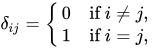
Suppose we are given a Hilbert space and a Hermitian operator over it called the Hamiltonian ${\displaystyle H}$. Ignoring complications about continuous spectra, we consider the discrete spectrum of ${\displaystyle H}$ and a basis of eigenvectors ${\displaystyle \{|\psi _{\lambda }\rangle \}}$ (see spectral theorem for Hermitian operators for the mathematical background): $${\displaystyle \left\langle \psi _{\lambda _{1}}|\psi _{\lambda _{2}}\right\rangle =\delta _{\lambda _{1}\lambda _{2}},}$$ where ${\displaystyle \delta _{ij}}$ is the Kronecker delta $${\displaystyle \delta _{ij}={\begin{cases}0&{\text{if }}i\neq j,\\1&{\text{if }}i=j,\end{cases}}}$$ and the ${\displaystyle \{|\psi _{\lambda }\rangle \}}$ satisfy the eigenvalue equation $${\displaystyle H\left|\psi _{\lambda }\right\rangle =\lambda \left|\psi _{\lambda }\right\rangle .}$$

Once again ignoring complications involved with a continuous spectrum of ${\displaystyle H}$, suppose the spectrum of ${\displaystyle H}$ is bounded from below and that its greatest lower bound is E₀. The expectation value of ${\displaystyle H}$ in a state ${\displaystyle |\psi \rangle }$ is then $${\displaystyle {\begin{aligned}\left\langle \psi \right|H\left|\psi \right\rangle &=\sum _{\lambda _{1},\lambda _{2}\in \mathrm {Spec} (H)}\left\langle \psi |\psi _{\lambda _{1}}\right\rangle \left\langle \psi _{\lambda _{1}}\right|H\left|\psi _{\lambda _{2}}\right\rangle \left\langle \psi _{\lambda _{2}}|\psi \right\rangle \\&=\sum _{\lambda \in \mathrm {Spec} (H)}\lambda \left|\left\langle \psi _{\lambda }|\psi \right\rangle \right|^{2}\geq \sum _{\lambda \in \mathrm {Spec} (H)}E_{0}\left|\left\langle \psi _{\lambda }|\psi \right\rangle \right|^{2}=E_{0}\langle \psi |\psi \rangle .\end{aligned}}}$$

If we were to vary over all possible states with norm 1 trying to minimize the expectation value of ${\displaystyle H}$, the lowest value would be ${\displaystyle E_{0}}$ and the corresponding state would be the ground state, as well as an eigenstate of ${\displaystyle H}$. Varying over the entire Hilbert space is usually too complicated for physical calculations, and a subspace of the entire Hilbert space is chosen, parametrized by some (real) differentiable parameters ${\displaystyle \alpha _{i}}$ (i = 1, 2, ..., N)}}. The choice of the subspace is called the ansatz. Some choices of ansatzes lead to better approximations than others, therefore the choice of ansatz is important.

Let's assume there is some overlap between the ansatz and the ground state (otherwise, it's a bad ansatz). We wish to normalize the ansatz, so we have the constraints $${\displaystyle \left\langle \psi (\mathbf {\alpha } )|\psi (\mathbf {\alpha } )\right\rangle =1}$$ and we wish to minimize $${\displaystyle \varepsilon (\mathbf {\alpha } )=\left\langle \psi (\mathbf {\alpha } )\right|H\left|\psi (\mathbf {\alpha } )\right\rangle .}$$

This, in general, is not an easy task, since we are looking for a global minimum and finding the zeroes of the partial derivatives of ${\displaystyle \varepsilon }$ over all ${\displaystyle \alpha _{i}}$ is not sufficient. If ${\displaystyle \psi (\alpha )}$ is expressed as a linear combination of other functions (${\displaystyle \alpha _{i}}$ being the coefficients), as in the Ritz method, there is only one minimum and the problem is straightforward. There are other, non-linear methods, however, such as the Hartree–Fock method, that are also not characterized by a multitude of minima and are therefore comfortable in calculations.

Although usually limited to calculations of the ground state energy, this method can be applied in certain cases to calculations of excited states as well. If the ground state wavefunction is known, either by the method of variation or by direct calculation, a subset of the Hilbert space can be chosen which is orthogonal to the ground state wavefunction.

$${\displaystyle \left|\psi \right\rangle =\left|\psi _{\text{test}}\right\rangle -\left\langle \psi _{\mathrm {gr} }|\psi _{\text{test}}\right\rangle \left|\psi _{\text{gr}}\right\rangle }$$

The resulting minimum is usually not as accurate as for the ground state, as any difference between the true ground state and ${\displaystyle \psi _{\text{gr}}}$ results in a lower excited energy. This defect is worsened with each higher excited state.

In another formulation: $${\displaystyle E_{\text{ground}}\leq \left\langle \phi \right|H\left|\phi \right\rangle .}$$

This holds for any trial ${\displaystyle \phi }$ since, by definition, the ground state wavefunction has the lowest energy, and any trial wavefunction will have energy greater than or equal to it.

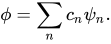
Proof: ${\displaystyle \phi }$ can be expanded as a linear combination of the actual eigenfunctions of the Hamiltonian (which we assume to be normalized and orthogonal): $${\displaystyle \phi =\sum _{n}c_{n}\psi _{n}.}$$

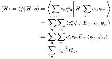
Then, to find the expectation value of the Hamiltonian: $${\displaystyle {\begin{aligned}\left\langle H\right\rangle =\left\langle \phi \right|H\left|\phi \right\rangle ={}&\left\langle \sum _{n}c_{n}\psi _{n}\right|H\left|\sum _{m}c_{m}\psi _{m}\right\rangle \\={}&\sum _{n}\sum _{m}\left\langle c_{n}^{*}\psi _{n}\right|E_{m}\left|c_{m}\psi _{m}\right\rangle \\={}&\sum _{n}\sum _{m}c_{n}^{*}c_{m}E_{m}\left\langle \psi _{n}|\psi _{m}\right\rangle \\={}&\sum _{n}|c_{n}|^{2}E_{n}.\end{aligned}}}$$

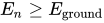
Now, the ground state energy is the lowest energy possible, i.e., ${\displaystyle E_{n}\geq E_{\text{ground}}}$. Therefore, if the guessed wave function ${\displaystyle \phi }$ is normalized: $${\displaystyle \left\langle \phi \right|H\left|\phi \right\rangle \geq E_{\text{ground}}\sum _{n}|c_{n}|^{2}=E_{\text{ground}}.}$$

For a Hamiltonian ${\displaystyle H}$ that describes the studied system and any normalizable function ${\displaystyle \Psi }$ with arguments appropriate for the unknown wave function of the system, we define the functional $${\displaystyle \varepsilon \left[\Psi \right]={\frac {\left\langle \Psi \right|{\hat {H}}\left|\Psi \right\rangle }{\left\langle \Psi |\Psi \right\rangle }}.}$$

The variational principle states that

• ${\displaystyle \varepsilon \geq E_{0}}$, where ${\displaystyle E_{0}}$ is the lowest energy eigenstate (ground state) of the hamiltonian
• ${\displaystyle \varepsilon =E_{0}}$ if and only if ${\displaystyle \Psi }$ is exactly equal to the wave function of the ground state of the studied system.

The variational principle formulated above is the basis of the variational method used in quantum mechanics and quantum chemistry to find approximations to the ground state.

Another facet in variational principles in quantum mechanics is that since ${\displaystyle \Psi }$ and ${\displaystyle \Psi ^{\dagger }}$ can be varied separately (a fact arising due to the complex nature of the wave function), the quantities can be varied in principle just one at a time.^[4]

The helium atom consists of two electrons with mass m and electric charge −e, around an essentially fixed nucleus of mass M ≫ m and charge +2e. The Hamiltonian for it, neglecting the fine structure, is: $${\displaystyle H=-{\frac {\hbar ^{2}}{2m}}\left(\nabla _{1}^{2}+\nabla _{2}^{2}\right)-{\frac {e^{2}}{4\pi \varepsilon _{0}}}\left({\frac {2}{r_{1}}}+{\frac {2}{r_{2}}}-{\frac {1}{|\mathbf {r} _{1}-\mathbf {r} _{2}|}}\right)}$$ where ħ is the reduced Planck constant, ε₀ is the vacuum permittivity, r_i (for i = 1, 2) is the distance of the i-th electron from the nucleus, and |r₁ − r₂| is the distance between the two electrons.

If the term V_ee = e²/(4πε₀|r₁ − r₂|), representing the repulsion between the two electrons, were excluded, the Hamiltonian would become the sum of two hydrogen-like atom Hamiltonians with nuclear charge +2e. The ground state energy would then be 8E₁ = −109 eV, where E₁ is the Rydberg constant, and its ground state wavefunction would be the product of two wavefunctions for the ground state of hydrogen-like atoms:^[2]: 262 $${\displaystyle \psi (\mathbf {r} _{1},\mathbf {r} _{2})={\frac {Z^{3}}{\pi a_{0}^{3}}}e^{-Z\left(r_{1}+r_{2}\right)/a_{0}}.}$$ where a₀ is the Bohr radius and Z = 2, helium's nuclear charge. The expectation value of the total Hamiltonian H (including the term V_ee) in the state described by ψ₀ will be an upper bound for its ground state energy. ⟨V_ee⟩ is −5E₁/2 = 34 eV, so ⟨H⟩ is 8E₁ − 5E₁/2 = −75 eV.

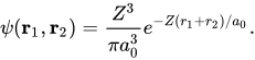
A tighter upper bound can be found by using a better trial wavefunction with 'tunable' parameters. Each electron can be thought to see the nuclear charge partially "shielded" by the other electron, so we can use a trial wavefunction equal with an "effective" nuclear charge Z < 2: The expectation value of H in this state is: $${\displaystyle \left\langle H\right\rangle =\left[-2Z^{2}+{\frac {27}{4}}Z\right]E_{1}}$$

This is minimal for Z = 27/16 implying shielding reduces the effective charge to ~1.69. Substituting this value of Z into the expression for H yields 729E₁/128 = −77.5 eV, within 2% of the experimental value, −78.975 eV.^[5]

Even closer estimations of this energy have been found using more complicated trial wave functions with more parameters. This is done in physical chemistry via variational Monte Carlo.

References

[edit]- ^ Sommerfeld, Thomas (2011-11-01). "Lorentz Trial Function for the Hydrogen Atom: A Simple, Elegant Exercise". Journal of Chemical Education. 88 (11): 1521–1524. Bibcode:2011JChEd..88.1521S. doi:10.1021/ed200040e. ISSN 0021-9584.
- ^ a b Griffiths, D. J. (1995). Introduction to Quantum Mechanics. Upper Saddle River, New Jersey: Prentice Hall. ISBN 978-0-13-124405-4.
- ^ Sakurai, J. J. (1994). Tuan, San Fu (ed.). Modern Quantum Mechanics (Revised ed.). Addison–Wesley. ISBN 978-0-201-53929-5.
- ^ see Landau, Quantum Mechanics, pg. 58 for some elaboration.
- ^ Drake, G.W.F.; Van, Zong-Chao (1994). "Variational eigenvalues for the S states of helium". Chemical Physics Letters. 229 (4–5). Elsevier BV: 486–490. Bibcode:1994CPL...229..486D. doi:10.1016/0009-2614(94)01085-4. ISSN 0009-2614.
Variational method (quantum mechanics)
View on GrokipediaIntroduction
Definition and Purpose
The variational method in quantum mechanics serves as an approximation technique to estimate the ground state energy of a quantum system, yielding an upper bound to the true eigenvalue through the use of trial wave functions. By selecting a suitable trial function and evaluating its expectation value with respect to the Hamiltonian operator, the method provides a calculable energy that is always greater than or equal to the exact ground state energy, allowing for systematic improvements by refining the trial function.[2] This approach is essential for addressing many-body problems in quantum chemistry and atomic physics, where the Schrödinger equation lacks exact analytical solutions due to the intricate correlations among multiple particles, such as electrons in atoms or molecules. It enables practical computations for systems that would otherwise be unsolvable, facilitating insights into molecular structures and reaction mechanisms.[5] In the broader context of computational quantum mechanics, the variational method underpins key algorithms, including the Hartree-Fock method, which applies variational optimization to a parameterized antisymmetrized product of single-particle orbitals to approximate the many-electron wave function and energy. At its core, the method systematically minimizes the expectation value of the Hamiltonian over a space of parameterized trial functions to achieve the tightest upper bound possible within that framework.[5]Historical Development
The variational method originated in the late 19th century with the work of Lord Rayleigh, who applied it in 1870 to approximate the fundamental frequency of vibration in an organ pipe closed at one end and open at the other, treating the problem as a classical wave phenomenon.[6] Rayleigh further developed this approach in 1873 for computing vibration frequencies of mechanical systems, establishing a foundational principle for minimizing energy functionals in continuous media.[5] In the early 20th century, Walther Ritz extended Rayleigh's ideas to a more general framework for solving eigenvalue problems in boundary value equations, publishing key papers in 1908 and 1909 that demonstrated procedures for approximating solutions to partial differential equations through variational minimization.[7] This extension, known as the Rayleigh-Ritz method, provided a systematic way to handle complex boundary conditions in mathematical physics. Ritz's contributions, completed before his death in 1909 at age 31, laid the groundwork for numerical approximations in diverse physical contexts.[8] Following the formulation of the Schrödinger equation in 1926, the variational method was rapidly adopted in quantum mechanics during the late 1920s for approximating solutions to the time-independent Schrödinger equation, with early applications focused on atomic spectra calculations.[9] A seminal quantum application came in 1929 when Egil A. Hylleraas used the method to compute the ground-state energy of the helium atom, achieving millihartree precision and demonstrating its power for multi-electron systems.[10] This work marked a pivotal integration of the variational approach into quantum theory, influencing subsequent developments in atomic physics.[11] The method evolved significantly in the mid-20th century with the advent of electronic computers in the 1950s and 1960s, transforming it from a manual approximation tool into a cornerstone of computational quantum chemistry.[12] During this period, researchers leveraged early computing resources to perform ab initio calculations, establishing foundations for large-scale simulations of molecular systems and solid-state properties.[13] By the 1960s, the variational method had become integral to quantum chemical computations, enabling more accurate predictions of electronic structures.[12]Theoretical Foundation
Variational Principle
The variational principle in quantum mechanics asserts that the ground state of a quantum system minimizes the expectation value of the energy among all possible states in the Hilbert space. This principle is rooted in the time-independent Schrödinger equation, $ H \phi = E \phi $, where $ H $ is the Hamiltonian operator, $ \phi $ is the exact eigenfunction corresponding to energy eigenvalue $ E $, and the ground state energy $ E_0 $ is the lowest such eigenvalue.[14][2] Formally, for any trial wave function $ \psi $ normalized such that $ \langle \psi | \psi \rangle = 1 $, the expectation value of the Hamiltonian satisfiesProof of the Upper Bound
The proof of the upper bound in the variational theorem relies on the spectral decomposition of the Hamiltonian operator , which is assumed to be Hermitian and thus possesses a complete, orthonormal set of eigenfunctions satisfying , where the eigenvalues are real and ordered such that .[17] Consider a normalized trial wave function (i.e., ), which can be expanded in the complete basis of eigenfunctions asFormulation and Implementation
Trial Wave Functions
In the variational method, trial wave functions serve as approximate representations of the true quantum mechanical wave function, designed to yield an upper bound to the ground state energy through minimization of the expectation value of the Hamiltonian. These functions are chosen to capture essential physical features of the system while remaining computationally tractable.[5] A good trial wave function must satisfy several key criteria to ensure its validity and effectiveness. It must be normalizable, meaning the integral of its squared magnitude over all space is finite, which guarantees a well-defined probability density. Additionally, it should obey the boundary conditions of the problem, such as vanishing at infinity for bound states, and incorporate relevant symmetries, including antisymmetry under particle exchange for fermionic systems to comply with the Pauli exclusion principle. The function should also exhibit the correct asymptotic behavior at large distances and smooth differentiability where the potential is finite, ensuring that the Hamiltonian operator applied to it yields convergent integrals.[18][5] To enable energy minimization, trial wave functions are typically parameterized with adjustable variables that allow flexibility in shape and extent. For instance, a variational parameter might scale the spatial extent, such as an effective width or charge-like term, which is varied to lower the energy expectation value. This parameterization balances accuracy with simplicity, as the optimal parameters are found by solving the condition that the derivative of the energy with respect to each parameter vanishes.[19][5] Common types of trial wave functions include simple analytic forms that mimic known exact solutions for simpler systems. Gaussian functions, of the form with normalization constant and parameter , are widely used due to their computational convenience in evaluating integrals. Slater-type orbitals, expressed as where is a variational exponent, provide exponential decay suitable for atomic-like systems. For multi-particle problems, trial functions often take the form of products of single-particle orbitals, potentially combined with correlation factors to account for interactions.[5][19][20] The quality of a trial wave function directly impacts the tightness of the upper bound on the ground state energy: more flexible and physically accurate forms, closer to the exact solution, produce lower variational energies but at the expense of increased computational cost due to more complex integrals or higher-dimensional parameter spaces. Optimization proceeds by iteratively adjusting parameters to minimize , often leveraging analytical derivatives for efficiency. In cases with multiple parameters, this process aligns with the Rayleigh-Ritz method for systematic improvement.[18][5]Rayleigh-Ritz Method
The Rayleigh-Ritz method is a systematic numerical technique for applying the variational principle to approximate the eigenvalues and eigenfunctions of the Hamiltonian operator in quantum mechanics, particularly for bound states. It involves expanding the trial wave function as a linear combination of a set of basis functions and optimizing the coefficients to minimize the energy expectation value. This approach, originally formulated for classical vibration problems by Lord Rayleigh in the late 19th century and extended to boundary value problems by Walter Ritz in 1909, was adapted to quantum mechanics in the early 20th century for solving the Schrödinger equation.[3][21] In the procedure, the trial wave function is expressed as a superposition , where forms a complete, linearly independent basis set spanning a subspace of the Hilbert space, and the coefficients are variational parameters. The goal is to minimize the Rayleigh quotient, defined as the expectation value of the Hamiltonian normalized by the norm of the trial function:where is the Hamiltonian matrix with elements , is the overlap matrix with , and is the column vector of coefficients. This minimization is performed subject to the normalization constraint .[22][23] Minimizing leads to a generalized eigenvalue problem , which can be solved by finding the roots of the secular determinant . The eigenvalues obtained from this equation provide upper bounds to the true eigenvalues of the Hamiltonian, with the lowest eigenvalue serving as an upper bound to the ground state energy. For non-orthogonal bases, the overlap matrix accounts for the non-orthogonality, ensuring the problem is well-posed even if the basis functions are not orthonormal.[22][23] The method's advantages lie in its systematic nature: increasing the basis set size enlarges the trial subspace, leading to progressively better approximations that converge monotonically from above to the exact eigenvalues as , provided the basis is complete. This convergence is guaranteed by the properties of the variational principle and the min-max theorem for Hermitian operators. The Rayleigh-Ritz approach is particularly effective for multi-parameter optimization, transforming the variational problem into a standard linear algebra task that scales favorably for moderate basis sizes in quantum chemical calculations.[22]