
Community hub
Recent from talks
Contribute something
Nothing was collected or created yet.
Convolutional code
View on WikipediaThis article needs additional citations for verification. (May 2015) |
In telecommunication, a convolutional code is a type of error-correcting code that generates parity symbols via the sliding application of a boolean polynomial function to a data stream. The sliding application represents the 'convolution' of the encoder over the data, which gives rise to the term 'convolutional coding'. The sliding nature of the convolutional codes facilitates trellis decoding using a time-invariant trellis. Time invariant trellis decoding allows convolutional codes to be maximum-likelihood soft-decision decoded with reasonable complexity.
The ability to perform economical maximum likelihood soft decision decoding is one of the major benefits of convolutional codes. This is in contrast to classic block codes, which are generally represented by a time-variant trellis and therefore are typically hard-decision decoded. Convolutional codes are often characterized by the base code rate and the depth (or memory) of the encoder . The base code rate is typically given as , where n is the raw input data rate and k is the data rate of output channel encoded stream. n is less than k because channel coding inserts redundancy in the input bits. The memory is often called the "constraint length" K, where the output is a function of the current input as well as the previous inputs. The depth may also be given as the number of memory elements v in the polynomial or the maximum possible number of states of the encoder (typically: ).
![{\displaystyle [n,k,K]}](https://wikimedia.org/api/rest_v1/media/math/render/svg/3b79e3732d617bcbd9cb5c8ab76e90da7de8b66c)


Convolutional codes are often described as continuous. However, it may also be said that convolutional codes have arbitrary block length, rather than being continuous, since most real-world convolutional encoding is performed on blocks of data. Convolutionally encoded block codes typically employ termination. The arbitrary block length of convolutional codes can also be contrasted to classic block codes, which generally have fixed block lengths that are determined by algebraic properties.
The code rate of a convolutional code is commonly modified via symbol puncturing. For example, a convolutional code with a 'mother' code rate may be punctured to a higher rate of, for example, simply by not transmitting a portion of code symbols. The performance of a punctured convolutional code generally scales well with the amount of parity transmitted. The ability to perform economical soft decision decoding on convolutional codes, as well as the block length and code rate flexibility of convolutional codes, makes them very popular for digital communications.


History
[edit]Convolutional codes were introduced in 1955 by Peter Elias. It was thought that convolutional codes could be decoded with arbitrary quality at the expense of computation and delay. In 1967, Andrew Viterbi determined that convolutional codes could be maximum-likelihood decoded with reasonable complexity using time invariant trellis based decoders — the Viterbi algorithm. Other trellis-based decoder algorithms were later developed, including the BCJR decoding algorithm.
Recursive systematic convolutional codes were invented by Claude Berrou around 1991. These codes proved especially useful for iterative processing including the processing of concatenated codes such as turbo codes.[1]
Using the "convolutional" terminology, a classic convolutional code might be considered a Finite impulse response (FIR) filter, while a recursive convolutional code might be considered an Infinite impulse response (IIR) filter.
Where convolutional codes are used
[edit]
Convolutional codes are used extensively to achieve reliable data transfer in numerous applications, such as digital video, radio, mobile communications (e.g., in GSM, GPRS, EDGE and 3G networks (until 3GPP Release 7)[3][4]) and satellite communications.[5] These codes are often implemented in concatenation with a hard-decision code, particularly Reed–Solomon. Prior to turbo codes such constructions were the most efficient, coming closest to the Shannon limit.
Convolutional encoding
[edit]To convolutionally encode data, start with k memory registers, each holding one input bit. Unless otherwise specified, all memory registers start with a value of 0. The encoder has n modulo-2 adders (a modulo 2 adder can be implemented with a single Boolean XOR gate, where the logic is: 0+0 = 0, 0+1 = 1, 1+0 = 1, 1+1 = 0), and n generator polynomials — one for each adder (see figure below). An input bit m1 is fed into the leftmost register. Using the generator polynomials and the existing values in the remaining registers, the encoder outputs n symbols. These symbols may be transmitted or punctured depending on the desired code rate. Now bit shift all register values to the right (m1 moves to m0, m0 moves to m−1) and wait for the next input bit. If there are no remaining input bits, the encoder continues shifting until all registers have returned to the zero state (flush bit termination).

The figure below is a rate 1⁄3 (m⁄n) encoder with constraint length (k) of 3. Generator polynomials are G1 = (1,1,1), G2 = (0,1,1), and G3 = (1,0,1). Therefore, output bits are calculated (modulo 2) as follows:
- n1 = m1 + m0 + m−1
- n2 = m0 + m−1
- n3 = m1 + m−1.
Convolutional codes can be systematic and non-systematic:
- systematic repeats the structure of the message before encoding
- non-systematic changes the initial structure
Non-systematic convolutional codes are more popular due to better noise immunity. It relates to the free distance of the convolutional code.[6]
-
 A short illustration of non-systematic convolutional code.
 -
 A short illustration of systematic convolutional code.


Recursive and non-recursive codes
[edit]The encoder on the picture above is a non-recursive encoder. Here's an example of a recursive one and as such it admits a feedback structure:

The example encoder is systematic because the input data is also used in the output symbols (Output 2). Codes with output symbols that do not include the input data are called non-systematic.
Recursive codes are typically systematic and, conversely, non-recursive codes are typically non-systematic. It isn't a strict requirement, but a common practice.
The example encoder in Img. 2. is an 8-state encoder because the 3 registers will create 8 possible encoder states (23). A corresponding decoder trellis will typically use 8 states as well.
Recursive systematic convolutional (RSC) codes have become more popular due to their use in Turbo Codes. Recursive systematic codes are also referred to as pseudo-systematic codes.
Other RSC codes and example applications include:

Useful for LDPC code implementation and as inner constituent code for serial concatenated convolutional codes (SCCC's).

Useful for SCCC's and multidimensional turbo codes.

Useful as constituent code in low error rate turbo codes for applications such as satellite links. Also suitable as SCCC outer code.
Impulse response, transfer function, and constraint length
[edit]A convolutional encoder is called so because it performs a convolution of the input stream with the encoder's impulse responses:
![{\displaystyle y_{i}^{j}=\sum _{k=0}^{\infty }h_{k}^{j}x_{i-k}=(x*h^{j})[i],}](https://wikimedia.org/api/rest_v1/media/math/render/svg/37626083236994588ffa49f06b4b3f8e05facffb)
where x is an input sequence, yj is a sequence from output j, hj is an impulse response for output j and denotes convolution.

A convolutional encoder is a discrete linear time-invariant system. Every output of an encoder can be described by its own transfer function, which is closely related to the generator polynomial. An impulse response is connected with a transfer function through Z-transform.
Transfer functions for the first (non-recursive) encoder are:


Transfer functions for the second (recursive) encoder are:


Define m by

where, for any rational function ,

- .

Then m is the maximum of the polynomial degrees of the
, and the constraint length is defined as . For instance, in the first example the constraint length is 3, and in the second the constraint length is 4.


Trellis diagram
[edit]A convolutional encoder is a finite state machine. An encoder with n binary cells will have 2n states.
Imagine that the encoder (shown on Img.1, above) has '1' in the left memory cell (m0), and '0' in the right one (m−1). (m1 is not really a memory cell because it represents a current value). We will designate such a state as "10". According to an input bit the encoder at the next turn can convert either to the "01" state or the "11" state. One can see that not all transitions are possible for (e.g., a decoder can't convert from "10" state to "00" or even stay in "10" state).
All possible transitions can be shown as below:

An actual encoded sequence can be represented as a path on this graph. One valid path is shown in red as an example.
This diagram gives us an idea about decoding: if a received sequence doesn't fit this graph, then it was received with errors, and we must choose the nearest correct (fitting the graph) sequence. The real decoding algorithms exploit this idea.
Free distance and error distribution
[edit]
The free distance[7] (d) is the minimal Hamming distance between different encoded sequences. The correcting capability (t) of a convolutional code is the number of errors that can be corrected by the code. It can be calculated as

Since a convolutional code doesn't use blocks, processing instead a continuous bitstream, the value of t applies to a quantity of errors located relatively near to each other. That is, multiple groups of t errors can usually be fixed when they are relatively far apart.
Free distance can be interpreted as the minimal length of an erroneous "burst" at the output of a convolutional decoder. The fact that errors appear as "bursts" should be accounted for when designing a concatenated code with an inner convolutional code. The popular solution for this problem is to interleave data before convolutional encoding, so that the outer block (usually Reed–Solomon) code can correct most of the errors.
Decoding convolutional codes
[edit]
Several algorithms exist for decoding convolutional codes. For relatively small values of k, the Viterbi algorithm is universally used as it provides maximum likelihood performance and is highly parallelizable. Viterbi decoders are thus easy to implement in VLSI hardware and in software on CPUs with SIMD instruction sets.
Longer constraint length codes are more practically decoded with any of several sequential decoding algorithms, of which the Fano algorithm is the best known. Unlike Viterbi decoding, sequential decoding is not maximum likelihood but its complexity increases only slightly with constraint length, allowing the use of strong, long-constraint-length codes. Such codes were used in the Pioneer program of the early 1970s to Jupiter and Saturn, but gave way to shorter, Viterbi-decoded codes, usually concatenated with large Reed–Solomon error correction codes that steepen the overall bit-error-rate curve and produce extremely low residual undetected error rates.
Both Viterbi and sequential decoding algorithms return hard decisions: the bits that form the most likely codeword. An approximate confidence measure can be added to each bit by use of the Soft output Viterbi algorithm. Maximum a posteriori (MAP) soft decisions for each bit can be obtained by use of the BCJR algorithm.
Popular convolutional codes
[edit]
![{\displaystyle h^{1}=171_{o}=[1111001]_{b}}](https://wikimedia.org/api/rest_v1/media/math/render/svg/1691b8f48b9ce15cbca503b5205617f49cf91312)
![{\displaystyle h^{2}=133_{o}=[1011011]_{b}}](https://wikimedia.org/api/rest_v1/media/math/render/svg/fffca9507c72d521bdeef60a5375cdd71d7b0d6d)

In fact, predefined convolutional codes structures obtained during scientific researches are used in the industry. This relates to the possibility to select catastrophic convolutional codes (causes larger number of errors).
An especially popular Viterbi-decoded convolutional code, used at least since the Voyager program, has a constraint length K of 7 and a rate r of 1/2.[12]
Mars Pathfinder, Mars Exploration Rover and the Cassini probe to Saturn use a K of 15 and a rate of 1/6; this code performs about 2 dB better than the simpler code at a cost of 256× in decoding complexity (compared to Voyager mission codes).

The convolutional code with a constraint length of 2 and a rate of 1/2 is used in GSM as an error correction technique.[13]
Punctured convolutional codes
[edit]
Convolutional code with any code rate can be designed based on polynomial selection;[15] however, in practice, a puncturing procedure is often used to achieve the required code rate. Puncturing is a technique used to make a m/n rate code from a "basic" low-rate (e.g., 1/n) code. It is achieved by deleting of some bits in the encoder output. Bits are deleted according to a puncturing matrix. The following puncturing matrices are the most frequently used:
| Code rate | Puncturing matrix | Free distance (for NASA standard K=7 convolutional code) | ||||||||||||||
|---|---|---|---|---|---|---|---|---|---|---|---|---|---|---|---|---|
| 1/2 (No perf.) |
|
10 | ||||||||||||||
| 2/3 |
|
6 | ||||||||||||||
| 3/4 |
|
5 | ||||||||||||||
| 5/6 |
|
4 | ||||||||||||||
| 7/8 |
|
3 |
For example, if we want to make a code with rate 2/3 using the appropriate matrix from the above table, we should take a basic encoder output and transmit every first bit from the first branch and every bit from the second one. The specific order of transmission is defined by the respective communication standard.
Punctured convolutional codes are widely used in the satellite communications, for example, in Intelsat systems and Digital Video Broadcasting.
Punctured convolutional codes are also called "perforated".
Turbo codes: replacing convolutional codes
[edit]
Simple Viterbi-decoded convolutional codes are now giving way to turbo codes, a new class of iterated short convolutional codes that closely approach the theoretical limits imposed by Shannon's theorem with much less decoding complexity than the Viterbi algorithm on the long convolutional codes that would be required for the same performance. Concatenation with an outer algebraic code (e.g., Reed–Solomon) addresses the issue of error floors inherent to turbo code designs.
See also
[edit]References
[edit] This article incorporates public domain material from Federal Standard 1037C. General Services Administration. Archived from the original on 2022-01-22.
- ^ Benedetto, Sergio, and Guido Montorsi. "Role of recursive convolutional codes in turbo codes." Electronics Letters 31.11 (1995): 858-859.
- ^ Eberspächer J. et al. GSM-architecture, protocols and services. John Wiley & Sons, 2008. p.97
- ^ 3rd Generation Partnership Project (September 2012). "3GGP TS45.001: Technical Specification Group GSM/EDGE Radio Access Network; Physical layer on the radio path; General description". Retrieved 2013-07-20.
- ^ Halonen, Timo, Javier Romero, and Juan Melero, eds. GSM, GPRS and EDGE performance: evolution towards 3G/UMTS. John Wiley & Sons, 2004. p. 430
- ^ Butman, S. A., L. J. Deutsch, and R. L. Miller. "Performance of concatenated codes for deep space missions." The Telecommunications and Data Acquisition Progress Report 42-63, March–April 1981 (1981): 33-39.
- ^ Moon, Todd K. "Error correction coding." Mathematical Methods and Algorithms. Jhon Wiley and Son (2005). p. 508
- ^ Moon, Todd K. "Error correction coding." Mathematical Methods and Algorithms. Jhon Wiley and Son (2005).- p.508
- ^ LLR vs. Hard Decision Demodulation (MathWorks)
- ^ Estimate BER for Hard and Soft Decision Viterbi Decoding (MathWorks)
- ^ Digital modulation: Exact LLR Algorithm (MathWorks)
- ^ Digital modulation: Approximate LLR Algorithm (MathWorks)
- ^ Butman, S. A., L. J. Deutsch, and R. L. Miller. "Performance of concatenated codes for deep space missions." The Telecommunications and Data Acquisition Progress Report 42-63, March–April 1981 (1981): 33-39.
- ^ Global system for mobile communications (GSM)
- ^ Punctured Convolutional Coding (MathWorks)
- ^ "Convert convolutional code polynomials to trellis description – MATLAB poly2trellis".
- ^ Turbo code
- ^ Benedetto, Sergio, and Guido Montorsi. "Role of recursive convolutional codes in turbo codes." Electronics Letters 31.11 (1995): 858-859.
External links
[edit]- The on-line textbook: Information Theory, Inference, and Learning Algorithms, by David J.C. MacKay, discusses convolutional codes in Chapter 48.
- The Error Correcting Codes (ECC) Page
- Matlab explanations
- Fundamentals of Convolutional Decoders for Better Digital Communications
- Convolutional codes (MIT)
- Information Theory and Coding (TU Ilmenau) Archived 2017-08-30 at the Wayback Machine, discusses convolutional codes on page 48.
Further reading
[edit]Publications
[edit]- Francis, Michael. "Viterbi Decoder Block Decoding-Trellis Termination and Tail Biting." Xilinx XAPP551 v2. 0, DD (2005): 1-21.
- Chen, Qingchun, Wai Ho Mow, and Pingzhi Fan. "Some new results on recursive convolutional codes and their applications." Information Theory Workshop, 2006. ITW'06 Chengdu. IEEE. IEEE, 2006.
- Fiebig, U-C., and Patrick Robertson. "Soft-decision and erasure decoding in fast frequency-hopping systems with convolutional, turbo, and Reed-Solomon codes." IEEE Transactions on Communications 47.11 (1999): 1646-1654.
- Bhaskar, Vidhyacharan, and Laurie L. Joiner. "Performance of punctured convolutional codes in asynchronous CDMA communications under perfect phase-tracking conditions." Computers & Electrical Engineering 30.8 (2004): 573-592.
- Modestino, J., and Shou Mui. "Convolutional code performance in the Rician fading channel." IEEE Transactions on Communications 24.6 (1976): 592-606.
- Chen, Yuh-Long, and Che-Ho Wei. "Performance evaluation of convolutional codes with MPSK on Rician fading channels." IEE Proceedings F-Communications, Radar and Signal Processing. Vol. 134. No. 2. IET, 1987.
Convolutional code
View on GrokipediaHistorical Development
Origins and Invention
Convolutional codes were invented by Peter Elias in 1955 at the Massachusetts Institute of Technology (MIT), where he was a faculty member working on advanced error-correcting techniques as part of broader research into sequential codes.[8] In his influential paper "Coding for Noisy Channels," Elias proposed these codes to enable reliable communication over noisy channels at rates approaching the theoretical limits established by information theory.[4] The development of convolutional codes was deeply motivated by Claude Shannon's 1948 noisy channel coding theorem, which demonstrated the existence of codes capable of achieving arbitrarily low error probabilities at rates up to the channel capacity, but did not provide explicit constructions.[9] Elias sought to bridge this gap by exploring continuous encoding methods that could handle streaming data, unlike the discrete block-based approaches dominant in early coding theory, thereby facilitating practical implementations for real-time transmission scenarios.[8] Elias initially described convolutional codes as linear time-varying codes with effectively infinite length, distinguishing them from fixed-length block codes by allowing the encoding process to incorporate memory across an unbounded sequence of symbols.[9] This structure enabled the generation of parity-check symbols through a convolutional operation, providing a flexible framework for error correction in continuous data flows. Early practical considerations for real-time error correction in data transmission emerged in the late 1950s at MIT's Lincoln Laboratory, where simulations and hardware prototypes laid the groundwork for deployable systems.[10] These efforts paved the way for later adoption in space communications.[11]Key Milestones and Adoption
The foundational work on convolutional code decoding was advanced by Andrew Viterbi in 1967, who established error bounds and introduced an asymptotically optimal maximum-likelihood decoding algorithm that became essential for practical implementation, although further refinements followed in subsequent years. In the 1960s, convolutional codes achieved their first major practical adoption through NASA's deep-space missions, notably employing a rate-1/2 code in the Pioneer program for telemetry data transmission over noisy interplanetary channels.[12] This application demonstrated the codes' robustness in extreme environments, paving the way for broader use in space communications. By the 1970s, integration into military systems accelerated reliability in secure links, as seen in standards like MIL-STD-188 for tactical radios, while early cellular prototypes explored their potential for mobile voice error correction.[13] The 1980s and 1990s marked widespread commercialization and standardization. GSM networks adopted a rate-1/2 convolutional code with constraint length k=5 to protect speech and signaling data against fading and interference, enabling reliable global mobile service rollout starting in 1991.[14] Concurrently, satellite applications proliferated, with GPS incorporating convolutional coding in its L1 C/A signal for navigation message integrity against atmospheric distortions.[15] A pivotal 1993 publication on Viterbi decoding optimizations further refined computational efficiency, directly shaping CCSDS recommendations for concatenated coding in space telemetry standards.[16]Overview and Fundamentals
Definition and Basic Principles
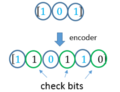
Convolutional codes constitute a class of error-correcting codes designed for digital communication systems, where each output symbol is generated as a linear function of a fixed number of consecutive input bits, referred to as a sliding window, thereby producing a continuous stream of encoded bits in contrast to the fixed-block structure of block codes.[17] This approach enables ongoing encoding without predefined message boundaries, making convolutional codes particularly suitable for streaming data transmission over noisy channels.[17] At their core, convolutional codes operate as linear time-invariant filters over the binary field GF(2), where the encoded output sequence is obtained by convolving the input bit sequence with a set of generator sequences that define the code's structure.[18] Theoretically, this convolution implies an infinite impulse response, as each input bit influences all subsequent outputs; however, practical implementations impose a finite memory constraint to bound computational complexity and ensure realizability with finite-state machines.[18] The linearity over GF(2) ensures that the superposition principle holds, allowing efficient decoding techniques based on algebraic properties.[18] A fundamental parameter of convolutional codes is the memory order , which specifies the number of previous input bits retained in the encoder's memory, leading to distinct internal states that track the memory contents at any encoding step.[19] The code rate quantifies the efficiency, indicating that input bits are mapped to output bits per encoding step, with typical values like providing redundancy for error correction at the cost of increased bandwidth.[17] For illustration, consider a rate-1/2 code with : processing the input sequence 10 (followed by two zero tail bits for termination) yields the output sequence 11 01 11 00, where each pair of output bits depends on the current input bit and the two prior bits stored in memory.[20]Comparison to Other Error-Correcting Codes
Convolutional codes differ fundamentally from block codes, such as Hamming and Reed-Solomon codes, in their encoding mechanism. Block codes operate on fixed-length input blocks to produce corresponding output codewords, relying on algebraic structures like parity-check matrices or polynomials defined over finite fields. In contrast, convolutional codes encode an input data stream continuously through a linear shift-register structure, where each output symbol depends not only on the current input but also on previous inputs via the code's memory, enabling ongoing processing without discrete block boundaries. This distinction makes convolutional codes more adaptable to streaming or variable-length data scenarios, whereas block codes necessitate buffering data into predefined blocks, which can introduce delays in continuous transmission systems.[21] A primary advantage of convolutional codes lies in their suitability for real-time and streaming applications, where the sequential nature of encoding and decoding allows for variable latency that aligns with ongoing data arrival, unlike the fixed-block processing of codes like Hamming, which may require complete block reception before correction. This flexibility is particularly beneficial in systems with large or indefinite data streams, such as satellite communications, where convolutional codes demonstrate superior energy efficiency and performance as block lengths or delays increase compared to traditional block codes. Moreover, convolutional codes are frequently integrated into hybrid error-correction schemes, where they serve as inner codes concatenated with outer block codes like Reed-Solomon; this combination exploits the burst-error resilience of Reed-Solomon with the random-error correction prowess of convolutional codes, enhancing overall system reliability in concatenated architectures.[21][22] Despite these strengths, convolutional codes have notable limitations relative to advanced block codes, particularly low-density parity-check (LDPC) codes. At low code rates, LDPC block codes generally outperform convolutional codes by approaching channel capacity more closely, achieving higher coding gains with lower error floors due to their sparse parity-check matrices and iterative message-passing decoding. Convolutional codes also exhibit greater sensitivity to burst errors, as their finite memory can propagate error bursts across the trellis; without additional interleaving to disperse errors into random patterns, their performance degrades significantly in bursty channels, in contrast to Reed-Solomon codes, which inherently correct bursts up to a designed length without interleaving.[23][24] In terms of performance, a standard rate-1/2 convolutional code with Viterbi decoding provides an asymptotic coding gain of approximately 5 dB at a bit error rate (BER) of compared to uncoded transmission over an additive white Gaussian noise channel, highlighting their effectiveness for moderate-rate applications, though gains diminish at very low rates relative to LDPC alternatives.[25]Applications
Communication Systems and Protocols
Convolutional codes play a crucial role in wireless communication systems, particularly in legacy cellular standards for protecting voice channels against errors in fading environments. In the Global System for Mobile Communications (GSM), the voice channels employ a rate-1/2 convolutional code with constraint length 7, defined by generator polynomials 133 and 171 in octal notation, to encode class 1 bits of the speech data, ensuring reliable transmission over noisy radio links.[26] Similarly, in Universal Mobile Telecommunications System (UMTS), convolutional coding with rates of 1/2 or 1/3 and constraint length 9—using generator polynomials 561 and 753 (octal) for rate 1/2, and 557, 663, 711 (octal) for rate 1/3—is applied to voice and control channels for forward error correction, enhancing speech quality in wideband code-division multiple access (W-CDMA) setups.[27] Early versions of the IEEE 802.11 Wi-Fi standards, such as 802.11a and 802.11g, integrate rate-1/2 convolutional codes with constraint length 7 and the same 133/171 generator polynomials at the physical layer to provide forward error correction for orthogonal frequency-division multiplexing (OFDM) signals, improving throughput in local area networks.[28] In satellite and deep space communications, convolutional codes are essential for mitigating signal attenuation and noise over vast distances. The NASA Deep Space Network (DSN) utilizes rate-1/2 convolutional codes with constraint length 7 for telemetry downlink, enabling robust data recovery from distant probes.[29] This configuration was notably employed in the Voyager missions, where the convolutional encoder processes high-rate data streams with a symbol rate twice the bit rate, concatenated with outer Reed-Solomon codes to achieve low bit error rates in the challenging interplanetary channel.[30] For wired telecommunications, convolutional codes provide error protection in environments susceptible to impulse noise and crosstalk. Digital subscriber line (DSL) modems, particularly asymmetric DSL (ADSL), incorporate convolutional codes as the inner layer of a concatenated scheme, often decoded via the Viterbi algorithm, to correct random errors in multicarrier-modulated signals transmitted over twisted-pair copper lines.[31] Integrated Services Digital Network (ISDN) systems similarly leverage convolutional-based trellis coding for error resilience in basic rate interfaces, safeguarding voice and data services against channel impairments in narrowband access networks.[32] A key protocol standardizing convolutional code usage is the Consultative Committee for Space Data Systems (CCSDS) TM Synchronization and Channel Coding recommendation (CCSDS 131.0-B), which mandates convolutional coding—typically rate-1/2 with constraint length 7—as the inner code in a concatenated architecture with an outer Reed-Solomon code (255,223) for telemetry applications, ensuring interoperability across space agencies for burst-error-prone links.Modern and Emerging Uses
In fifth-generation (5G) New Radio (NR) systems, convolutional codes have been proposed in hybrid schemes with low-density parity-check (LDPC) codes for ultra-reliable low-latency communication (URLLC) scenarios, integrating sequential error correction with iterative decoding to achieve reliability targets below 10^{-5} packet error rate under stringent latency constraints of 1 ms.[33] Such hybrids address the challenges of short codewords in industrial IoT and vehicular applications by optimizing error floors and convergence in belief propagation decoding. In Internet of Things (IoT) networks, lightweight convolutional code variants are employed in low-power protocols to enhance reliability in battery-constrained environments. Bluetooth Low Energy (BLE), as defined in the Bluetooth Core Specification version 5.0 and later, incorporates rate-1/3 convolutional forward error correction (FEC) in its LE Coded PHY mode, operating at 500 kbps or 125 kbps to extend range and robustness against interference while minimizing computational overhead.[34] This non-systematic, non-recursive code with constraint length 4 uses generator polynomials (7, 5, 7 in octal) to protect payload data, enabling error rates below 10^{-3} in fading channels typical of wearable and sensor devices. For Zigbee-based systems adhering to IEEE 802.15.4, convolutional coding has been proposed as a variant to improve transceiver performance in mesh networks, with rate-1/8 codes demonstrating up to 3 dB coding gain over uncoded schemes in simulations for energy-efficient home automation.[35] These adaptations prioritize Viterbi decoding complexity under 10^4 operations per frame to preserve battery life exceeding 5 years in typical deployments. Convolutional codes are integrated into quantum key distribution (QKD) protocols for error correction in noisy quantum channels, where quantum convolutional codes provide continuous protection for qubit streams without requiring block synchronization. These codes, constructed via stabilizer formalism on infinite lattices, correct phase and bit-flip errors in continuous-variable QKD systems. In optical communications, convolutional codes enhance forward error correction in fiber-optic systems, particularly when paired with multilevel modulation schemes like 16-QAM, yielding bit error rates below 10^{-9} at signal-to-noise ratios 2-3 dB below uncoded thresholds in long-haul terrestrial links.[36] Rate-1/2 non-systematic convolutional encoders with Viterbi decoding are favored for their adaptability to soft-decision inputs from coherent receivers, supporting data rates up to 100 Gbps in dense wavelength-division multiplexing (DWDM) setups. Convolutional codes continue to be explored for real-time video streaming applications, providing error resilience in unreliable wireless links using punctured rate-1/2 variants to add redundancy. In hybrid configurations, convolutional encoding precedes video codecs to provide burst-error correction for low-latency applications such as augmented reality, where decoding latency is constrained to under 20 ms on resource-limited edge nodes. This stems from the codes' efficient hardware implementation on field-programmable gate arrays, suitable for scenarios with variable channel conditions. As of 2025, convolutional codes are also proposed in 6G research for massive IoT and concatenated with polar/LDPC codes in updated space data systems like CCSDS for enhanced satellite IoT reliability.[37]Encoding Process
Generator Polynomials and Shift Registers
The encoder for a convolutional code is typically implemented using a shift register architecture with m memory elements, where m = K - 1 and K is the constraint length. This structure functions as a linear feedback shift register (LFSR), where each new input bit enters the register and causes the existing contents to shift, typically to the right. Specific positions in the register, known as taps—including the current input and selected memory elements—are connected to modulo-2 adders (XOR gates) to produce the output bits according to the generator polynomials. This setup ensures that the output depends on the current input and the previous m input bits stored in memory.[17] Generator polynomials specify the tap connections and are binary polynomials over GF(2), often represented in octal notation for compactness. For a rate-1/n code, there are n such polynomials, denoted g^{(i)}(D) for i = 1 to n, where D represents the delay operator. The overall encoder is described by the generator matrix in polynomial form G(D) = [g^{(1)}(D) \ g^{(2)}(D) \ \dots \ g^{(n)}(D)]. A widely adopted example is the rate-1/2 code with constraint length K=7, known as the NASA standard for deep-space communications, using g^{(1)}(D) = 1 + D^3 + D^4 + D^5 + D^6 (octal 171) and g^{(2)}(D) = 1 + D + D^3 + D^4 + D^6 (octal 133). These polynomials correspond to binary representations 1111001 and 1011011, respectively, where the least significant bit is the coefficient of D^0 (current input) and the most significant bit is for D^6 (oldest memory).[38] The outputs are computed via convolution of the input sequence with each generator polynomial, modulo 2. In the time domain, for input sequence {u_j} (with u_j = 0 for j < 0), the i-th output bit at time j is \begin{equation*} v_j^{(i)} = \sum_{l=0}^{m} u_{j-l} , g_l^{(i)} \pmod{2}, \quad i = 1, \dots, n. \end{equation*} This equation captures the linear combination of the current and past inputs weighted by the polynomial coefficients g_l^{(i)}.[17] For the rate-1/2, K=7 code with polynomials (171, 133)_8, the encoding of input 101 (with initial register state all zeros) proceeds as follows, using the coefficients g_l^{(1)} = [1, 0, 0, 1, 1, 1, 1] and g_l^{(2)} = [1, 1, 0, 1, 1, 0, 1] (l = 0 to 6). At each step, the register holds the last 6 inputs, and outputs are XOR sums over the taps.| Step (j) | Input u_j | Register state after shift (u_j, u_{j-1}, ..., u_{j-6}) | v_j^{(1)} calculation (sum mod 2) | v_j^{(2)} calculation (sum mod 2) | Output (v_j^{(1)} v_j^{(2)}) |
|---|---|---|---|---|---|
| 0 | 1 | 1 0 0 0 0 0 0 | 1·1 + 0·0 + 0·0 + 1·0 + 1·0 + 1·0 + 1·0 = 1 | 1·1 + 1·0 + 0·0 + 1·0 + 1·0 + 0·0 + 1·0 = 1 | 11 |
| 1 | 0 | 0 1 0 0 0 0 0 | 1·0 + 0·1 + 0·0 + 1·0 + 1·0 + 1·0 + 1·0 = 0 | 1·0 + 1·1 + 0·0 + 1·0 + 1·0 + 0·0 + 1·0 = 1 | 01 |
| 2 | 1 | 1 0 1 0 0 0 0 | 1·1 + 0·0 + 0·1 + 1·0 + 1·0 + 1·0 + 1·0 = 1 | 1·1 + 1·0 + 0·1 + 1·0 + 1·0 + 0·0 + 1·0 = 1 | 11 |
Systematic vs. Non-Systematic Encoding
In non-systematic convolutional encoding, all output bits are generated as linear combinations of the current and past input bits stored in shift registers, without directly reproducing the input sequence in any output stream. This approach, often realized through feedforward shift register structures with modulo-2 addition based on generator polynomials, yields codewords where the original message is fully obscured in the encoded form.[1] For instance, a common rate-1/2 non-systematic code uses generator polynomials , producing outputs and , where is the input polynomial.[1] Such codes typically achieve a higher free distance , enhancing error-correcting performance, but data recovery necessitates complete decoding of the entire sequence since the input is not explicitly present.[39] Systematic convolutional encoding, by contrast, incorporates the input bit stream unchanged as one or more of the output streams, supplemented by parity bits derived from linear combinations of the input and shift register contents. This structure simplifies partial data extraction, as the original message can be read directly from the systematic output without full error correction, which is advantageous for applications requiring low-latency access to information bits.[1] However, including the input directly often results in a lower minimum distance compared to equivalent non-systematic codes, potentially reducing overall coding gain.[19] For a rate-1/2 systematic code, the generators might take the form , ensuring the first output matches the input while the second provides redundancy.[1] In general, for a rate- code, the systematic generator matrix is structured as , where is the identity matrix and is a polynomial matrix generating the parity outputs.[39] The choice between systematic and non-systematic forms involves key trade-offs in performance and complexity. Non-systematic codes offer superior minimum distance and coding gain—for example, a non-systematic rate-1/2 code with constraint length 3 can achieve , yielding a coding gain or approximately 4 dB—but require more involved decoding to retrieve data.[1] Systematic codes, while potentially sacrificing some distance (e.g., reduced due to the unprotected input stream), enable delay-free encoding, non-catastrophic behavior, and minimal realizations, making them preferable for systems prioritizing encoding simplicity and partial decoding efficiency.[1] Systematic forms are employed in various communication standards where these benefits outweigh the performance penalty, such as in certain wireless protocols that value straightforward implementation.[17] Every convolutional code admits both systematic and non-systematic realizations, allowing transformation between them via algebraic operations on the generator matrix. To convert a non-systematic code to systematic, assuming the leading generator has constant term 1, one premultiplies the generator tuple by , yielding new generators where the first is 1 and others are adjusted accordingly; this preserves the code's overall properties while altering the encoding structure.[1] For multi-input codes, reordering outputs or inverting submatrices of can achieve the systematic form .[39] These conversions are typically performed during code design using shift register implementations, ensuring equivalence in the generated code space.[1]Code Architectures
Non-Recursive (Feedforward) Codes
Non-recursive, or feedforward, convolutional codes produce output symbols through linear combinations of the current input bit and past input bits stored in a shift register, achieved via connections known as taps, with no feedback path altering the input sequence.[40] This structure relies on finite impulse response (FIR) filtering, where each output branch computes a modulo-2 sum of selected input bits based on the tap positions.[1] The mathematical representation uses a time-invariant generator matrix , a matrix whose entries are polynomials in the formal delay variable , corresponding to the coefficients of the FIR filters in each branch.[39] For an input sequence represented as a polynomial , the output codeword polynomial is , yielding a rate code where the degree of the polynomials determines the memory order.[40] Feedforward codes simplify hardware realization, as their acyclic structure eliminates feedback loops, enabling straightforward implementation with shift registers and adders without the need for recursive state updates.[1] Additionally, they mitigate catastrophic error propagation—where finite input errors produce infinite output errors—by choosing non-catastrophic generator polynomials; for rate codes, this requires the greatest common divisor of all generator polynomials to be 1.[39] A representative example is the rate , constraint length 3 feedforward code with generator polynomials (octal 7) and (octal 5), which is non-catastrophic since .[40] This code, widely adopted in early communication standards, demonstrates the tap-based structure with two output branches and a 2-bit memory.[5]Recursive (Feedback) Codes
Recursive (feedback) codes, also known as recursive convolutional codes, incorporate a feedback mechanism in their encoder structure, where the input path depends on previous states through a recursive loop. This creates a dependence on prior inputs, typically implemented using a shift register with feedback connections that modify the input to the register based on a linear combination of past states modulo 2. Unlike feedforward codes, this recursion introduces a dynamic memory effect that propagates information indefinitely.[1] The generator functions for recursive codes are expressed in rational form, with the feedback polynomial appearing in the denominator of the transfer function. For instance, a simple rate-1/2 recursive code can have a transfer function such as , where the denominator represents the feedback path. In systematic recursive form, the output includes the unmodified input alongside the recursive parity bits, enhancing decodability.[1] These codes exhibit an infinite impulse response due to the feedback loop, which contrasts with the finite response of non-recursive structures and can lead to longer error events. They offer potential for achieving higher free distance compared to equivalent non-systematic codes, improving error correction capability, but poorly designed feedback polynomials risk generating catastrophic codes, where finite input errors propagate to infinite decoding errors.[41] Recursive systematic convolutional codes play a pivotal role as constituent components in turbo codes, where their recursive nature facilitates effective iterative decoding by producing high-weight codewords from low-weight inputs. A common example uses the feedback polynomial , corresponding to octal representation 13, paired with a feedforward polynomial for the parity output.[41]Structural Properties
Constraint Length and Memory
In convolutional coding, the constraint length is a fundamental parameter that quantifies the memory inherent in the encoder structure. It is defined as , where represents the maximum memory order or the number of memory elements (such as shift register stages) in the encoder. This means that each output symbol depends on the current input bit and up to previous input bits, spanning a total of consecutive input bits.[17] The constraint length thus measures the "window" of input history that influences the encoding process, directly tying into the shift register implementation where past bits are stored to compute linear combinations via generator polynomials.[42] For a general rate convolutional code, the constraint length is typically the same for all inputs and defined as , where is the memory order per input stream, ensuring that the encoder's memory is captured consistently across branches.[42] For binary rate 1/n convolutional codes (typically over GF(2)), the number of encoder states equals , as each state is defined by the content of the memory elements holding the previous input bits.[17] The choice of constraint length embodies a key trade-off in convolutional code design: larger enhances error-correcting performance by increasing redundancy and allowing detection of longer error patterns, but it exponentially raises decoding complexity due to the growing number of states. For instance, a rate code with (thus ) yields 64 states, a configuration that provides robust performance in practical systems like satellite communications while remaining feasible for Viterbi decoding, with each trellis branch reflecting transitions over the -bit input span.[17] This balance has made moderate constraint lengths like to prevalent in standards, prioritizing achievable computational demands over marginal gains from very large .[42]Impulse Response and Transfer Function
The impulse response of a convolutional code characterizes the output sequence produced by the encoder in response to a unit impulse input, typically a single '1' bit followed by an infinite sequence of '0' bits. For a rate-1/n binary convolutional encoder, the impulse response is an n-tuple of sequences, each corresponding to one output branch, and its length is finite for non-recursive (feedforward) encoders, determined by the memory order , but infinite for recursive encoders due to feedback loops that prevent the state from returning to zero in finite time.[1] The transfer function provides a frequency-domain (or z-transform) representation of the encoder's behavior, expressed as , where is the numerator polynomial and is the denominator polynomial, both with coefficients in the finite field (e.g., ). For feedforward encoders, the transfer function simplifies to , a polynomial generator with , reflecting the finite impulse response. In recursive encoders, feedback introduces a non-trivial denominator , making a rational function that captures the infinite impulse response.[1] These representations enable analysis of code properties, such as computing codeweight enumerators, which count the number of codewords of each weight to evaluate error-correcting performance. The transfer function generates output sequences as , where is the input polynomial, allowing enumeration of low-weight paths in the code trellis.[1][43] A representative example is the rate-1/2 convolutional code with generator polynomials in octal notation (5,7), corresponding to and , with memory order . The impulse response yields output pairs: (1,1) at time 0, (0,1) at time 1, and (1,1) at time 2, followed by zeros, confirming the finite length tied to the memory. The transfer function is , used to derive weight enumerators for this feedforward code.[43]Graphical Representations
Trellis Diagrams
Trellis diagrams provide a graphical representation of the state transitions in a convolutional encoder over time, illustrating the possible sequences of states and outputs for a given code. In this structure, nodes represent the possible memory states of the encoder, with the number of states equal to , where is the memory order. The horizontal axis denotes time steps or input symbols, while branches connect states at consecutive time instants, labeled with the input bit and the corresponding output symbols generated during the transition. This construction captures the convolutional nature of the code by repeating a basic section, known as a trellis section, for each input symbol, forming an infinite or finite (for terminated codes) lattice-like diagram.[44] Valid codewords correspond to paths through the trellis starting from the all-zero initial state and, for terminated codes, ending at the all-zero state after a finite length. Each path traces a unique sequence of branches, where merging paths between states highlight the code's redundancy, as multiple input sequences may converge to the same state, enforcing error-detecting properties. The divergence and subsequent merging of paths from a common state represent potential error events, visualizing how the code separates distinct messages over time.[44] A representative example is the trellis for a rate-1/2 convolutional code with memory , yielding 4 states labeled as 00, 01, 10, and 11 (in binary, representing shift register contents). At each time step, an input bit of 0 or 1 causes transitions: for instance, from state 00, input 0 leads to state 00 with output 00, while input 1 leads to state 10 with output 11 (assuming standard generator polynomials). Branches from other states follow similarly, with the diagram showing parallel branches for each input possibility, forming a symmetric pattern that repeats across time. This 4-state trellis demonstrates how inputs drive state evolution, with outputs appended along the path to form the codeword.[45] Trellis diagrams serve as the foundational structure for efficient decoding algorithms, enabling systematic exploration of all possible code paths to identify the most likely transmitted sequence. In particular, they facilitate the Viterbi algorithm by allowing dynamic programming over the states, reducing computational complexity from exponential to linear in the number of branches per state. For codes with higher initial constraint lengths , the trellis exhibits butterfly-like structures in early sections, reflecting the initial state uncertainty before settling into the periodic pattern.[44]State Diagrams
State diagrams offer a compact graphical representation of convolutional encoders as finite-state machines, capturing the evolution of the encoder's memory states without the time dimension inherent in trellis diagrams. Each node corresponds to a possible state of the shift registers, typically 2^{m} nodes for a code with memory order m, where the state is labeled by the binary content of the registers (e.g., "00", "01"). Directed edges connect states based on the next input bit, with labels indicating the input symbol and the resulting output symbols computed via the generator polynomials; for a rate-1/n code, each edge is annotated as input/output tuple, such as 0/00 or 1/11. This construction directly follows from the shift-register implementation, where advancing the state involves shifting in the new input bit and generating outputs as linear combinations modulo 2.[42][46] For analytical purposes, particularly in deriving code performance metrics, a modified state diagram is employed. In this version, the all-zero state is split into a source node (initial state) and a sink node (final state), with no self-loop on the source; all other transitions form loops that may return to the sink. Edges are relabeled with variables tracking key properties: D raised to the Hamming weight of the output branch, N (or I) to the power of the number of input 1's on that branch, and optionally J (or L) for the branch length in symbols. This split-loop structure isolates paths from the source to the sink, representing divergent error events that start and end in the zero state, while excluding the all-zero path. The diagram's topology reveals cycles corresponding to code loops, with self-loops at non-zero states for zero-input transitions and cross-connections driven by input 1's.[42][47] A representative example is the rate-1/2 convolutional code with constraint length K=3 (m=2), using generator polynomials g_1(D) = 1 + D + D^2 (octal 7) and g_2(D) = 1 + D^2 (octal 5). The four states are 00, 01, 10, and 11. From state 00, input 0 yields output 00 and stays at 00 (self-loop); input 1 yields 11 and goes to 10. From 01, input 0 goes to 00 with 11; input 1 to 10 with 00. From 10, input 0 to 01 with 10; input 1 to 11 with 01. From 11, input 0 to 01 with 01; input 1 to 11 with 10 (self-loop). In the modified version, the source connects only to non-zero states via input-1 branches, with loops like the self-loop at 11 labeled N D^1 J (for input 1, output 10) and cross-links such as from 10 to 11 labeled N D^1 J (input 1, output 01). This illustrates the split from source, loops among {01,10,11}, and returns to sink.[42][46][20] These diagrams are instrumental in computing generating functions that enumerate error events. By applying Mason's gain formula or solving systems of linear equations from the branch gains (e.g., the transfer function T(D,N) = \sum N^{w_i} D^{w_o} over paths from source to sink, where w_i and w_o are input and output weights), the diagram yields the input-output weight enumerating function, which bounds bit and event error probabilities and identifies the free distance as the minimum exponent of D. This approach, foundational to performance analysis, relies on the diagram's acyclic paths in the modified form to sum contributions from all possible error cycles.[42][47]Performance Metrics
Free Distance
The free distance of a convolutional code is defined as the minimum Hamming weight among all nonzero code sequences produced by the encoder.[48] Due to the linearity of convolutional codes, this is equivalent to the minimum distance between any two distinct codewords.[49] This parameter serves as a primary indicator of the code's error-correcting capability, as larger values of enable the detection and correction of more errors before decoding failure occurs.[1] The free distance can be computed using the state diagram of the code or its transfer function, which enumerates the weights of paths that start and end at the zero state while diverging from the all-zero sequence.[1] For instance, the widely used rate-1/2 convolutional code with constraint length 7 and octal generators (171, 133), adopted as a NASA standard for deep-space communications, has a free distance of 10.[50] Algorithms based on modified Viterbi searches or generating functions facilitate this calculation, though they scale poorly with code complexity.[51] In terms of performance, the free distance bounds the number of correctable errors at approximately , following the general sphere-packing principle for linear codes.[1] Asymptotically, at high signal-to-noise ratios, the coding gain achieved by the code is given by dB, where is the code rate; for the (171, 133) code, this yields about 7 dB.[52] The free distance typically increases with the constraint length , enhancing error correction, but larger exponentially raises the computational demands for both encoding and distance evaluation due to the growing state space.[51]Error Events and Distribution
In convolutional codes, an error event refers to a finite-length path in the trellis that diverges from the all-zero reference path (corresponding to the transmitted codeword) and subsequently remerges with it. The length of such an event is measured by the number of branches from the divergence point to the remerge point, while the weight is the Hamming weight of the output symbols along that path, representing the number of differing bits relative to the all-zero sequence. These events model the typical decoding errors in maximum-likelihood decoding, where the decoder selects an incorrect path segment before correcting back to the true path.[1] The statistical distribution of error events is captured by the weight enumerator , where denotes the number of error events with output weight and input weight (the number of 1s in the input sequence causing the event). This enumerator enumerates all possible low-probability paths starting and ending at the zero state in the trellis, excluding the all-zero path itself. It is derived from the code's transfer function , a generating function obtained by modifying the state diagram: branches are labeled with terms , where and are the output and input weights of the branch, respectively; the transfer function is then computed as the rational expression , with and being polynomials from solving the system of linear equations for state variables (or equivalently, via the adjacency matrix inversion for the zero-state to zero-state paths). The coefficients of directly yield the , providing the spectrum of event weights and lengths essential for performance prediction.[53][54] This distribution enables upper bounds on error performance, such as the union bound on the bit error rate , where is the number of input bits per branch, , is the code rate, is the signal-to-noise ratio per bit, and the bound approximates the dominant low-weight events at high SNR (with higher-order terms involving the full spectrum for tighter estimates) for binary codes over AWGN channels with coherent BPSK modulation. The dominant term is .[1][5] For a rate-1/2 convolutional code with constraint length (4 memory elements, 16 states), the transfer function method enumerates low-weight error events by computing the generating function coefficients up to a desired degree, revealing the spectrum starting from the free distance (typically 7 for optimal generators like octal (53,75)). For instance, the minimum-weight events correspond to simple input sequences like a single 1 followed by zeros, yielding one event of weight 7; subsequent coefficients show increasing multiplicities for weights 8 and 9 (e.g., two events of weight 8 from length-5 paths), which dominate the error floor in performance curves. This enumeration highlights how longer events contribute less to the bound at high SNR but affect finite-length behavior.[53]Decoding Methods
Viterbi Algorithm
The Viterbi algorithm, introduced in 1967, is a maximum-likelihood decoding technique for convolutional codes that uses dynamic programming to identify the most probable transmitted sequence by finding the path through the trellis with the minimum cumulative metric.[55] This path corresponds to the codeword that minimizes the overall discrepancy between the received sequence and the expected outputs along the trellis branches.[56] The metric is computed as the Hamming distance for hard-decision decoding (counting bit errors) or the Euclidean distance for soft-decision decoding (using signal amplitudes).[56] The algorithm operates iteratively over the trellis time steps via the add-compare-select (ACS) operation: for each state, the path metrics from its two predecessor states are added to the respective branch metrics (differences between received and expected symbols), the two resulting values are compared, and the smaller one is selected as the new path metric for that state, with the predecessor pointer stored.[56] Survivor paths—pointers indicating the chosen predecessor for each state—are maintained at every time step to track the best path to each state, effectively pruning less likely alternatives and retaining only 2^m paths (one per state).[57] Upon completing all time steps for the received sequence of length n, traceback begins from the final state with the minimum path metric, following the survivor pointers backward to the initial state (typically the zero state) to reconstruct the input bit sequence.[56] The computational complexity of the standard Viterbi algorithm is O(2^m n), arising from processing 2^m states at each of the n time steps, with a constant number of add, compare, and select operations per state.[56] For sequential decoding variants, which aim to reduce average complexity below the fixed bound of Viterbi, pruning techniques such as the Fano algorithm can be applied by exploring promising paths in a depth-first manner and backtracking when metrics exceed thresholds.[55] A simple example illustrates the process for a rate-1/2 convolutional code with memory m=2 (constraint length K=3) and generator polynomials g1 = (1 + D + D^2) and g2 = (1 + D^2), often denoted in octal as (7,5). The trellis has 4 states (00, 01, 10, 11), with each input bit driving transitions that output two parity bits. Suppose the received sequence (after hard decisions) is 11 10 11 00 01 10, corresponding to 3 input bits over 6 time steps. Initialize path metrics at time 0: PM(00) = 0, PM(others) = ∞. At time 1 (received 11), expected outputs from state 00 are 00 (input 0) or 11 (input 1); branch metrics are Hamming distances (2 for 11 vs. 00 to state 00, 0 for 11 vs. 11 to state 10). Proceed with ACS operations over the time steps to update path metrics and store predecessors. Traceback from the final state with the minimum path metric reconstructs the most likely input bit sequence, detecting and correcting errors where the minimum metric exceeds zero.[57]Other Decoding Techniques
Sequential decoding represents an early approach to decoding convolutional codes with reduced average computational complexity compared to exhaustive search methods, though it incurs variable latency. Introduced by Wozencraft in the late 1950s, this technique performs a depth-first search through the code tree or trellis, prioritizing paths based on a metric that approximates the likelihood of the received sequence. The Fano algorithm, developed by Robert M. Fano in 1963, implements sequential decoding without requiring a stack by using a heuristic to backtrack and advance through promising branches, ensuring progress toward the most likely codeword while bounding the search depth to control complexity. This results in an average number of computations per decoded bit that is independent of the code length for rates below capacity, but performance degrades with higher error rates due to potential deep backtracks, leading to unbounded delays in worst cases. The stack algorithm, proposed by James L. Massey in 1969, addresses some of Fano's limitations by maintaining a stack of partial paths ordered by their metrics, allowing a more systematic exploration that reduces the risk of excessive backtracking and achieves near-maximum-likelihood performance with lower variance in computation time. Both variants offer significant complexity savings over the Viterbi algorithm for long codes, particularly in high-rate scenarios, but their variable latency makes them less suitable for real-time applications without additional buffering.[58] Threshold decoding provides a simpler, low-complexity alternative suitable for convolutional codes with short constraint lengths, relying on feedback correction rather than full path search. Developed by James L. Massey in 1963, this method treats the code as a set of orthogonal parity checks and decodes by computing syndrome bits and applying majority-logic thresholds to estimate information bits iteratively. For a rate-1/2 code with constraint length 3, threshold decoding can correct all single errors within a decoding window using a single-pass feedback loop, achieving performance close to maximum-likelihood decoding for low error rates while requiring only O(K) operations per bit, where K is the constraint length. Its simplicity stems from avoiding trellis storage, making it attractive for hardware implementation in early systems, though it is suboptimal for longer codes or higher noise levels, as error propagation in the feedback can amplify miscorrections. Threshold decoding is particularly effective for self-orthogonal convolutional codes designed with coset leaders, where the minimum distance bounds the correctable error patterns explicitly. The BCJR algorithm, also known as the maximum a posteriori (MAP) decoder, computes soft outputs for convolutional codes by performing forward and backward recursions on the trellis, providing symbol or bit probabilities essential for concatenated coding schemes. Named after its inventors Bahl, Cocke, Jelinek, and Raviv, this method was introduced in 1974 and calculates the posterior probability of each state or transition given the entire received sequence, using the forward-backward algorithm to marginalize over all paths. Unlike hard-decision decoders, BCJR produces log-likelihood ratios for each bit, enabling reliable extrinsic information exchange in iterative systems, with computational complexity comparable to the Viterbi algorithm at O(2^K) per time step for constraint length K. For a standard rate-1/2 code with K=5, simulations show that BCJR achieves bit error rates within 0.5 dB of the Shannon limit when used in turbo-like configurations, highlighting its role in modern error correction despite the added forward pass. Its soft-output capability makes it foundational for approximate decoding in parallel concatenated codes, though exact implementation requires normalization to avoid underflow in probability computations. Approximate decoding techniques like the M-algorithm and T-algorithm reduce the complexity of maximum-likelihood search by pruning the trellis, trading a small performance loss for substantial computational savings in high-dimensional state spaces. The M-algorithm, a breadth-first approximation, retains only the M most likely paths at each stage of the trellis, discarding others to limit memory and operations to O(M \cdot 2^{K-1}) per branch, where M is typically much smaller than the full state count. For M=64 on a K=7 rate-1/2 code, this yields a 1-2 dB degradation in signal-to-noise ratio at 10^{-5} bit error rate compared to full Viterbi, while reducing complexity by over an order of magnitude, making it viable for bandwidth-constrained channels. The T-algorithm, a depth-first variant, prunes paths whose metrics fall below a dynamic threshold relative to the best path, allowing adaptive control of the search space and achieving similar performance with even lower average complexity, especially at high signal-to-noise ratios where few paths compete. These methods are particularly useful for real-time decoding of longer convolutional codes, balancing the exponential growth in Viterbi's requirements with near-optimal error rates through careful selection of M or threshold parameters.Standard and Variant Codes
Popular Rate-1/2 Codes
One of the most widely adopted rate-1/2 convolutional codes is the NASA Deep Space Network (DSN) standard, featuring a constraint length of K=7 and generator polynomials represented in octal as (171, 133). This code achieves a free distance d_free of 10, providing robust error correction suitable for deep space communications where signal attenuation is severe. It was employed in landmark missions including Voyager and Galileo to ensure reliable data transmission over vast distances.[59][60] In mobile communications, the Global System for Mobile Communications (GSM) utilizes a rate-1/2 convolutional code with constraint length K=5 for encoding speech data in the full-rate traffic channel (TCH/FS). The generator polynomials are G_0(D) = 1 + D^3 + D^4 and G_1(D) = 1 + D + D^3 + D^4, corresponding to octal notations (23, 35). This configuration yields a free distance of 7, balancing coding gain with encoder complexity for real-time voice transmission.[14] Another notable example is the code specified in the CCITT (now ITU-T) V.32 modem standard, which employs a rate-1/2 convolutional code with constraint length K=3 and generator polynomials in octal (5, 7). With a free distance of 5, this code supports trellis-coded modulation at data rates up to 9600 bps over telephone lines, enhancing reliability against noise and intersymbol interference.[61] These codes exemplify optimized designs for their respective applications, where performance is evaluated primarily through bit error rate (BER) in additive white Gaussian noise (AWGN) channels under Viterbi decoding. Coding gains typically range from 3 to 5 dB at BER=10^{-5}, depending on constraint length, with longer K offering diminishing returns due to increased decoding complexity. The table below summarizes free distances for optimal rate-1/2 binary convolutional codes across common constraint lengths.| Constraint Length (K) | Free Distance (d_free) |
|---|---|
| 3 | 5 |
| 4 | 6 |
| 5 | 7 |
| 6 | 8 |
| 7 | 10 |
| 8 | 12 |