Hubbry Logo
Data parallelismData parallelismMain
Open search
Data parallelism
Community hub
Data parallelism
logo
8 pages, 0 posts
0 subscribers
Be the first to start a discussion here.
Data parallelism
Data parallelism
from Wikipedia
Sequential vs. data-parallel job execution

Data parallelism is parallelization across multiple processors in parallel computing environments. It focuses on distributing the data across different nodes, which operate on the data in parallel. It can be applied on regular data structures like arrays and matrices by working on each element in parallel. It contrasts to task parallelism as another form of parallelism.

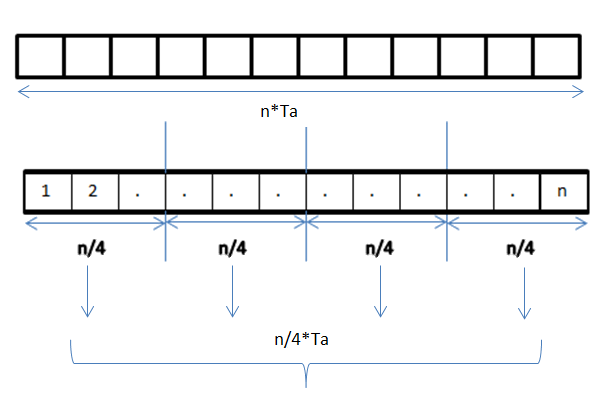
A data parallel job on an array of n elements can be divided equally among all the processors. Let us assume we want to sum all the elements of the given array and the time for a single addition operation is Ta time units. In the case of sequential execution, the time taken by the process will be n×Ta time units as it sums up all the elements of an array. On the other hand, if we execute this job as a data parallel job on 4 processors the time taken would reduce to (n/4)×Ta + merging overhead time units. Parallel execution results in a speedup of 4 over sequential execution. The locality of data references plays an important part in evaluating the performance of a data parallel programming model. Locality of data depends on the memory accesses performed by the program as well as the size of the cache.

History

[edit]

Exploitation of the concept of data parallelism started in 1960s with the development of the Solomon machine.[1] The Solomon machine, also called a vector processor, was developed to expedite the performance of mathematical operations by working on a large data array (operating on multiple data in consecutive time steps). Concurrency of data operations was also exploited by operating on multiple data at the same time using a single instruction. These processors were called 'array processors'.[2] In the 1980s, the term was introduced [3] to describe this programming style, which was widely used to program Connection Machines in data parallel languages like C*. Today, data parallelism is best exemplified in graphics processing units (GPUs), which use both the techniques of operating on multiple data in space and time using a single instruction.

Most data parallel hardware supports only a fixed number of parallel levels, often only one. This means that within a parallel operation it is not possible to launch more parallel operations recursively, and means that programmers cannot make use of nested hardware parallelism. The programming language NESL was an early effort at implementing a nested data-parallel programming model on flat parallel machines, and in particular introduced the flattening transformation that transforms nested data parallelism to flat data parallelism. This work was continued by other languages such as Data Parallel Haskell and Futhark, although arbitrary nested data parallelism is not widely available in current data-parallel programming languages.

Description

[edit]

In a multiprocessor system executing a single set of instructions (SIMD), data parallelism is achieved when each processor performs the same task on different distributed data. In some situations, a single execution thread controls operations on all the data. In others, different threads control the operation, but they execute the same code.

For instance, consider matrix multiplication and addition in a sequential manner as discussed in the example.

Example

[edit]

Below is the sequential pseudo-code for multiplication and addition of two matrices where the result is stored in the matrix C. The pseudo-code for multiplication calculates the dot product of two matrices A, B and stores the result into the output matrix C.

If the following programs were executed sequentially, the time taken to calculate the result would be of the (assuming row lengths and column lengths of both matrices are n) and for multiplication and addition respectively.

// Matrix multiplication
for (int i = 0; i < A.rowLength(); i++) {	
    for (int k = 0; k < B.columnLength(); k++) {
        int sum = 0;
        for (int j = 0; j < A.columnLength(); j++) {
            sum += A[i][j] * B[j][k];
        }
        C[i][k] = sum;
    }
}
// Array addition
for (int i = 0; i < c.size(); i++) {
    c[i] = a[i] + b[i];
}

We can exploit data parallelism in the preceding code to execute it faster as the arithmetic is loop independent. Parallelization of the matrix multiplication code is achieved by using OpenMP. An OpenMP directive, "omp parallel for" instructs the compiler to execute the code in the for loop in parallel. For multiplication, we can divide matrix A and B into blocks along rows and columns respectively. This allows us to calculate every element in matrix C individually thereby making the task parallel. For example: A[m x n] dot B [n x k] can be finished in instead of when executed in parallel using m*k processors.

Data parallelism in matrix multiplication
// Matrix multiplication in parallel
#pragma omp parallel for schedule(dynamic,1) collapse(2)
for (int i = 0; i < A.rowLength(); i++) {
    for (int k = 0; k < B.columnLength(); k++) {
        int sum = 0;
        for (int j = 0; j < A.columnLength(); j++) {
            sum += A[i][j] * B[j][k];
        }
        C[i][k] = sum;
    }
}

It can be observed from the example that a lot of processors will be required as the matrix sizes keep on increasing. Keeping the execution time low is the priority but as the matrix size increases, we are faced with other constraints like complexity of such a system and its associated costs. Therefore, constraining the number of processors in the system, we can still apply the same principle and divide the data into bigger chunks to calculate the product of two matrices.[4]

For addition of arrays in a data parallel implementation, let's assume a more modest system with two central processing units (CPU) A and B, CPU A could add all elements from the top half of the arrays, while CPU B could add all elements from the bottom half of the arrays. Since the two processors work in parallel, the job of performing array addition would take one half the time of performing the same operation in serial using one CPU alone.

The program expressed in pseudocode below—which applies some arbitrary operation, foo, on every element in the array d—illustrates data parallelism:[nb 1]

if CPU = "a" then
    lower_limit := 1
    upper_limit := round(d.length / 2)
else if CPU = "b" then
    lower_limit := round(d.length / 2) + 1
    upper_limit := d.length

for i from lower_limit to upper_limit by 1 do
    foo(d[i])

In an SPMD system executed on 2 processor system, both CPUs will execute the code.

Data parallelism emphasizes the distributed (parallel) nature of the data, as opposed to the processing (task parallelism). Most real programs fall somewhere on a continuum between task parallelism and data parallelism.

Steps to parallelization

[edit]

The process of parallelizing a sequential program can be broken down into four discrete steps.[5]

Type Description
Decomposition The program is broken down into tasks, the smallest exploitable unit of concurrence.
Assignment Tasks are assigned to processes.
Orchestration Data access, communication, and synchronization of processes.
Mapping Processes are bound to processors.

Data parallelism vs. task parallelism

[edit]
Data parallelism Task parallelism
Same operations are performed on different subsets of same data. Different operations are performed on the same or different data.
Synchronous computation Asynchronous computation
Speedup is more as there is only one execution thread operating on all sets of data. Speedup is less as each processor will execute a different thread or process on the same or different set of data.
Amount of parallelization is proportional to the input data size. Amount of parallelization is proportional to the number of independent tasks to be performed.
Designed for optimum load balance on multi processor system. Load balancing depends on the availability of the hardware and scheduling algorithms like static and dynamic scheduling.

Data parallelism vs. model parallelism

[edit]
Data parallelism Model parallelism
Same model is used for every thread but the data given to each of them is divided and shared. Same data is used for every thread, and model is split among threads.
It is fast for small networks but very slow for large networks since large amounts of data needs to be transferred between processors all at once. It is slow for small networks and fast for large networks.
Data parallelism is ideally used in array and matrix computations and convolutional neural networks Model parallelism finds its applications in deep learning

[6]

Mixed data and task parallelism

[edit]

Data and task parallelism, can be simultaneously implemented by combining them together for the same application. This is called Mixed data and task parallelism. Mixed parallelism requires sophisticated scheduling algorithms and software support. It is the best kind of parallelism when communication is slow and number of processors is large.[7]

Mixed data and task parallelism has many applications. It is particularly used in the following applications:

  1. Mixed data and task parallelism finds applications in the global climate modeling. Large data parallel computations are performed by creating grids of data representing Earth's atmosphere and oceans and task parallelism is employed for simulating the function and model of the physical processes.
  2. In timing based circuit simulation. The data is divided among different sub-circuits and parallelism is achieved with orchestration from the tasks.

Data parallel programming environments

[edit]

A variety of data parallel programming environments are available today, most widely used of which are:

  1. Message Passing Interface: It is a cross-platform message passing programming interface for parallel computers. It defines the semantics of library functions to allow users to write portable message passing programs in C, C++ and Fortran.
  2. OpenMP:[8] It's an Application Programming Interface (API) which supports shared memory programming models on multiple platforms of multiprocessor systems. Since version 4.5, OpenMP is also able to target devices other than typical CPUs. It can program FPGAs, DSPs, GPUs and more. It is not confined to GPUs like OpenACC.
  3. CUDA and OpenACC: CUDA and OpenACC (respectively) are parallel computing API platforms designed to allow a software engineer to utilize GPUs' computational units for general purpose processing.
  4. Threading Building Blocks and RaftLib: Both open source programming environments that enable mixed data/task parallelism in C/C++ environments across heterogeneous resources.

Applications

[edit]

Data parallelism finds its applications in a variety of fields ranging from physics, chemistry, biology, material sciences to signal processing. Sciences imply data parallelism for simulating models like molecular dynamics,[9] sequence analysis of genome data [10] and other physical phenomenon. Driving forces in signal processing for data parallelism are video encoding, image and graphics processing, wireless communications [11] to name a few.

Data-intensive computing

[edit]
Data-intensive computing is a class of parallel computing applications which use a data parallel approach to process large volumes of data typically terabytes or petabytes in size and typically referred to as big data. Computing applications that devote most of their execution time to computational requirements are deemed compute-intensive, whereas applications are deemed data-intensive if they require large volumes of data and devote most of their processing time to input/output and manipulation of data.[12]

See also

[edit]

Notes

[edit]

References

[edit]
Revisions and contributorsEdit on WikipediaRead on Wikipedia
from Grokipedia
Data parallelism is a fundamental technique in parallel computing that involves distributing data across multiple processors or computing devices, where each processes a distinct subset of the data using the same algorithm or model simultaneously to achieve faster execution. In this approach, the computational workload is divided by partitioning the input data rather than the program logic, enabling scalable performance on systems ranging from multi-core CPUs to large GPU clusters. This method originated in the 1980s with the rise of SIMD (Single Instruction, Multiple Data) architectures and data-parallel programming models for massively parallel machines, such as those with thousands of processors. In , particularly for training deep neural networks, data parallelism replicates the entire model across multiple devices—such as GPUs—while splitting the training batch into portions for independent forward and backward passes on each replica. After local computations, gradients are synchronized across devices, often using all-reduce operations, to update the model parameters collectively and maintain consistency. This synchronization step, inspired by early parameter-averaging techniques like those developed by , ensures that all model replicas converge to the same state despite processing different data subsets. Distributed implementations, such as PyTorch's DistributedDataParallel or 's framework, optimize this process to minimize communication overhead. Compared to model parallelism, which partitions the model itself across devices to handle large architectures that exceed single-device memory, data parallelism is simpler to implement and scales efficiently with data volume but requires the full model to fit on each device. Its advantages include linear in time for large datasets, ease of integration into existing frameworks, and broad applicability in distributed scenarios, though it can introduce bottlenecks from gradient synchronization in very large-scale setups. Today, data parallelism underpins much of modern AI on cloud platforms like Azure and AWS SageMaker, enabling the development of complex models at scale.

Fundamentals

Definition and Principles

Data parallelism is a paradigm in which the same operation is applied simultaneously to multiple subsets of a large across multiple processors or nodes, emphasizing the division of rather than tasks to enable concurrent execution of identical computations on different portions. This approach treats the , such as an , as globally accessible, with each processor operating on a distinct partition. In contexts, processors denote the hardware units—such as CPU cores or nodes in a cluster—that execute instructions independently. Threads represent lightweight sequences of instructions that share the same within a processor, facilitating fine-grained parallelism. In contrast, architectures assign private memory to each processor, necessitating explicit communication mechanisms, like , for exchange between them. Central principles of data parallelism revolve around data partitioning, , and load balancing. Data partitioning involves horizontally splitting the dataset into subsets, often using strategies like block distribution—where contiguous chunks are assigned to processors—or cyclic distribution—to promote even locality and minimize communication overhead. occurs at key points to aggregate results, typically through reduction operations such as sum or all-reduce, which combine partial computations from all processors into a unified global result, ensuring consistency in distributed environments. Load balancing is critical to distribute these partitions evenly across processors, preventing imbalances that could lead to time and suboptimal performance, particularly in systems with variable workload characteristics. The benefits of data parallelism include enhanced as dataset sizes grow, allowing additional processors to process larger volumes without linearly increasing execution time, and straightforward implementation for problems—those requiring minimal inter-task communication, such as independent data transformations. It enables potential linear speedup, governed by , which quantifies the theoretical maximum acceleration from parallelization. is expressed as S=1(1P)+PNS = \frac{1}{(1 - P) + \frac{P}{N}} where PP is the fraction of the total computation that can be parallelized, and NN is the number of processors; this formula highlights how speedup approaches 1/(1P)1/(1 - P) as NN increases, underscoring the importance of minimizing serial components for effective scaling.

Illustrative Example

To illustrate data parallelism, consider a simple scenario where the goal is to compute the sum of all elements in a large , such as one containing 1,000 numerical values, using four processors. The is partitioned into four equal of 250 elements each, with one assigned to each processor, exemplifying the principle of data partitioning where the workload is divided based on the data. In the first step, data distribution occurs: Processor 1 receives elements 1 through 250, Processor 2 receives 251 through 500, Processor 3 receives 501 through 750, and Processor 4 receives 751 through 1,000. Next, local computation takes place in parallel, with each processor independently summing the values in its assigned to produce a partial sum—for instance, Processor 1 might compute a partial sum of 12,500 from its elements. The process then involves communication for aggregation: The four partial sums are combined using an all-reduce operation, where each processor shares its result with the others, and all processors collectively compute the total sum (e.g., 50,000 if the partial sums add up accordingly). This yields the final result, the sum of the entire array, distributed across the processors for efficiency. A descriptive flow of this process can be outlined as follows:
  1. Initialization: Load the full on a master node and broadcast the partitioning scheme to all processors.
  2. Distribution: Scatter subsets to respective processors (e.g., via a scatter operation).
  3. Parallel Summation: Each processor computes its local sum without inter-processor communication.
  4. Reduction: Gather partial sums and reduce them (e.g., via all-reduce) to obtain the global , then broadcast the result if needed.
One common pitfall in such examples is an uneven data split, such as assigning 300 elements to one processor and 200 to another, which can lead to load imbalance where some processors idle while others finish later, reducing overall efficiency; this is mitigated by ensuring balanced partitioning as per core data parallelism principles.

Historical Development

Origins in Early Computing

In the mid-1960s, the theoretical foundations of data parallelism emerged within computer architecture classifications. Michael J. Flynn introduced his influential taxonomy in 1966, categorizing systems based on instruction and data streams, with the Single Instruction, Multiple Data (SIMD) class directly embodying data parallelism by applying one instruction to multiple data elements concurrently. This framework highlighted SIMD as a mechanism for exploiting inherent parallelism in array-based computations, distinguishing it from sequential single-data processing. Flynn's classification provided a conceptual blueprint for architectures that could handle bulk data operations efficiently, influencing subsequent designs in parallel computing. Key theoretical insights into parallel processing limits further shaped early understandings of data parallelism. In 1967, published a seminal arguing that while multiprocessor systems could accelerate parallelizable workloads, inherent sequential bottlenecks would cap overall gains, emphasizing the need to maximize the parallel fraction in data-intensive tasks. Concurrently, programming paradigms began supporting data-parallel ideas through array-oriented languages. Kenneth E. Iverson's 1962 work on APL ( established arrays as primitive types, enabling concise expressions for operations over entire datasets, such as vector additions or matrix transformations, which inherently promoted parallel evaluation. Early proposals like Daniel Slotnick's SOLOMON project in 1962 laid groundwork for SIMD architectures. By the mid-1970s, hardware innovations realized these concepts in practice. The , operational from 1974, was the first massively parallel computer with up to 256 processing elements executing SIMD instructions on array data. The supercomputer, delivered in 1976, incorporated vector registers and pipelines that performed SIMD-like operations on streams of data, allowing scientific simulations to process large arrays in parallel for enhanced throughput in fields like . This vector processing capability marked an early milestone in hardware support for data parallelism, bridging theoretical models with tangible performance improvements in batch-oriented scientific workloads.

Key Milestones and Evolution

The 1980s marked the rise of data parallelism through the development of massively parallel processors, exemplified by the introduced by in 1985. This SIMD-based architecture enabled simultaneous operations on large datasets across thousands of simple processors, facilitating efficient data-parallel computations for applications like simulations and image processing. Building on early SIMD concepts from vector processors, these systems demonstrated the of data parallelism for handling massive data volumes in a single instruction stream. In the , efforts toward standardization laid the groundwork for distributed data parallelism, culminating in the (MPI) standard released in 1994 by the MPI Forum. MPI provided a portable framework for message-passing in parallel programs across clusters, enabling data partitioning and communication in distributed-memory environments. The and 2000s saw further integration of data parallelism into (HPC) clusters, such as systems built from commodity hardware, which scaled to thousands of nodes for parallel . GPU acceleration accelerated this evolution with NVIDIA's platform launched in 2006, allowing programmers to write data-parallel kernels that exploit thousands of GPU cores for tasks like matrix operations and scientific simulations. The 2010s expanded data parallelism to large-scale distributed systems, influenced by big data frameworks such as , released in 2006, which implemented the model for fault-tolerant parallel processing of petabyte-scale datasets across clusters. This was complemented by in 2010, which introduced in-memory data parallelism via Resilient Distributed Datasets (RDDs), enabling faster iterative computations over distributed data compared to disk-based approaches. By the late 2010s and early 2020s, data parallelism evolved toward hybrid models integrating , where frameworks like Spark and MPI facilitate elastic scaling across cloud resources for dynamic workloads. Standards advanced with 5.0 in 2018, introducing enhanced support for task and data parallelism, including device offloading to accelerators and improved loop constructs for heterogeneous systems.

Implementation Approaches

Steps for Parallelization

To convert a sequential program into a data-parallel one, the process begins by analyzing the computational structure to ensure suitability for distribution across multiple processors, focusing on operations that can be applied uniformly to independent subsets. This involves a systematic sequence of steps that emphasize decomposition, , and coordination to achieve efficient parallelism while minimizing overheads such as communication and costs. The first step is to identify parallelizable portions of the program, particularly loops or iterations where computations on elements are independent and can be executed without interdependencies. For instance, operations like element-wise computations, as in summing an , are ideal candidates since each point can be processed separately. This identification requires profiling the code to locate computational hotspots and verify the absence of data races or sequential constraints. Next, partition the data into subsets that can be distributed across processors, using methods such as block distribution—where contiguous chunks of data are assigned to each processor—or cyclic distribution, which interleaves data elements round-robin style to balance load and improve locality. Block partitioning suits regular access patterns, while cyclic helps mitigate imbalances in irregular workloads by ensuring even computational distribution. The choice depends on data size, access patterns, and hardware topology to optimize memory access and reduce contention. Following partitioning, assign computations to processors by mapping data subsets to available compute units, ensuring that each processor handles its local portion with minimal global coordination. This mapping aligns data locality with processor architecture, such as assigning blocks to cores in a multicore system or nodes in a cluster, to maximize cache efficiency and pipeline utilization. Tools like MPI can facilitate this assignment through rank-based indexing. Subsequently, implement communication mechanisms to exchange necessary between processors, such as shared inputs at the start or using gather and reduce operations to aggregate outputs like partial sums. These operations ensure consistency without excessive data movement; for example, in a distributed sum, local results are reduced globally via . Efficient communication patterns, often via message-passing interfaces, are critical to avoid bottlenecks in distributed environments. Finally, handle synchronization to coordinate processors and manage errors, employing barriers to ensure all tasks complete phases before proceeding and incorporating through checkpointing or to recover from failures. Barriers prevent premature access to incomplete data, while fault tolerance mechanisms like periodic saves maintain progress in long-running computations. This step safeguards correctness and reliability in scalable systems. Success of data parallelization is evaluated using metrics like —the ratio of sequential to parallel execution time—and efficiency, which accounts for resource utilization. These are bounded by , which highlights that parallel gains are limited by the fraction of the program that remains sequential.

Programming Environments and Tools

Data parallelism implementations rely on a variety of programming environments and tools tailored to different hardware architectures and application scales. Traditional frameworks laid the groundwork for both distributed and shared-memory systems, while GPU-specific and modern distributed libraries have evolved to address the demands of large-scale , particularly in . The (MPI), first standardized in 1994 by the MPI Forum, serves as a foundational tool for distributed-memory data parallelism across clusters of computers. MPI enables explicit communication between processes, supporting data partitioning and synchronization through primitives like point-to-point sends/receives and collective operations such as MPI_Allreduce, which aggregates results from parallel computations. This makes it suitable for domain decomposition approaches where data is divided among nodes, with implementations like MPICH and OpenMPI providing portable, high-performance support for scalability up to thousands of processes. For shared-memory systems, , introduced in as an specification by a including and , uses simple directives to parallelize data-intensive loops on multi-core processors. Key directives like #pragma omp parallel for distribute loop iterations across threads, implicitly handling data sharing and load balancing in a fork-join model. OpenMP's directive-based approach minimizes code changes from serial programs, achieving good scalability on symmetric multiprocessors (SMPs) with low overhead for thread creation and synchronization. GPU-focused tools emerged to exploit the massive thread-level parallelism of graphics processing units. NVIDIA's Compute Unified Device Architecture (), released in 2006, provides a C/C++-like extension for writing kernels that execute thousands of threads in SIMD fashion over data arrays. 's hierarchical model—organizing threads into blocks and grids—facilitates efficient data parallelism by mapping computations to the GPU's streaming multiprocessors, with built-in for host-device data transfer. This has enabled speedups of orders of magnitude for workloads, though it is vendor-specific to hardware. Complementing CUDA, the Open Computing Language (OpenCL), standardized by the in , offers a cross-vendor alternative for heterogeneous parallelism on GPUs, CPUs, and accelerators. OpenCL kernels define parallel work-items grouped into work-groups, supporting data parallelism through vectorized operations and shared local memory, with platform portability across devices from , , and others. Its runtime handles command queues and buffering, reducing overhead in multi-device setups. Modern distributed frameworks, particularly for , build on these foundations to simplify multi-node data parallelism. PyTorch's DistributedDataParallel (DDP), part of the torch.distributed backend introduced in 2017 and refined in versions up to 2.9.1 (2025), wraps models for synchronous training across GPUs and nodes. DDP automatically partitions minibatches, performs all-reduce using NCCL or Gloo backends, and overlaps communication with to achieve near-linear on clusters of up to hundreds of GPUs. PyTorch and TensorFlow support multi-GPU setups with heterogeneous NVIDIA GPUs like RTX 5090 and RTX 2080 Ti via DataParallel, DistributedDataParallel (DDP), or manual device assignment; this is possible despite differing VRAM or compute capabilities, though with warnings about memory imbalances requiring careful management. Additionally, PyTorch provides Fully Sharded Data Parallel (FSDP), an advanced data-parallel technique that shards model parameters, optimizer states, and gradients across devices to significantly reduce per-device memory usage. This enables the training of very large models that exceed single-device memory capacity while maintaining the synchronization and scalability benefits of data parallelism. FSDP builds on DDP principles but adds sharding for memory efficiency, making it suitable for large-scale AI models. TensorFlow's tf.distribute , launched in 2019 with TensorFlow 2.0, provides high-level strategies for data parallelism, including MirroredStrategy for intra-node multi-GPU replication and MultiWorkerMirroredStrategy for cross-node distribution. It abstracts synchronization via collective ops like all-reduce, supporting and mixed-precision training with minimal code modifications. Horovod, open-sourced by in 2017, extends data parallelism across frameworks like and by integrating ring-allreduce algorithms over MPI or NCCL, enabling efficient gradient averaging with low bandwidth overhead. Horovod's design emphasizes framework interoperability and elastic scaling, achieving up to 90% efficiency on large GPU clusters compared to single-node training. As of 2025, however, Horovod is less actively maintained, with its last major release in 2023 and deprecation in certain platforms such as Azure . Among recent developments, Ray—initiated in 2016 by UC Berkeley researchers—incorporates data-parallel actors for stateful, distributed task execution, with updates from 2023 to 2025 enhancing fault-tolerant scaling for AI pipelines through improved actor scheduling and integration with Ray Train for parallel model training. In October 2025, Ray was transferred to the Foundation by Anyscale, enhancing its alignment with the broader ecosystem. Ray's actor model allows data-parallel operations on remote objects, supporting dynamic resource allocation across clusters. Dask, a flexible Python library for since 2015, received enhancements through 2025, including in version 2025.11.0 with joint optimization for multiple Dask-Expr backed collections, optimized for distributed arrays, and better GPU support via CuPy integration, streamlining data-parallel workflows in scientific computing. These updates reduce scheduling overhead and improve interoperability with libraries like and Pandas for out-of-core . Selecting among these tools involves evaluating trade-offs in communication overhead, , and ease of use. Lower overhead, as in Horovod's ring-allreduce, minimizes latency in gradient synchronization for distributed . is assessed via metrics like strong scaling efficiency, where tools like MPI and DDP maintain up to thousands of nodes by balancing and communication. Ease of use favors directive-based () or wrapper-style (DDP, tf.distribute) APIs that require few code alterations, enhancing developer productivity over low-level .

Comparative Analysis

Versus Task Parallelism

Task parallelism involves dividing a computational workload into distinct, independent tasks that are executed concurrently across multiple processors, with the data typically shared or replicated among them rather than partitioned. This approach contrasts with data parallelism by focusing on , where different operations or stages of a are assigned to separate processing units, often aligning with multiple-instruction, multiple-data (MIMD) architectures in . In MIMD systems, processors execute varied instructions on shared data sets, enabling flexibility for workflows with inherent task dependencies. Key differences between data parallelism and lie in their workload division strategies and synchronization requirements. Data parallelism partitions a large into subsets, applying the identical task—such as a or —to each subset simultaneously, resembling single-instruction, multiple-data (SIMD) execution for uniform operations. In contrast, assigns different tasks to processors operating on the same or overlapping data, necessitating dependency management to ensure correct ordering and avoid race conditions, whereas data parallelism primarily requires aggregation mechanisms like reduction operations to combine results. These distinctions influence scalability: data parallelism excels in scenarios with minimal inter-subset dependencies, while handles sequential or interdependent phases more naturally. Data parallelism offers advantages for uniform, large-scale datasets where the workload can scale with processor count, as illustrated by , which posits that speedup improves as problem size grows proportionally to the number of processors, countering Amdahl's fixed-problem limitations in task-oriented setups. However, it may underutilize resources if subsets vary in size or computation time, leading to load imbalance. , conversely, suits heterogeneous workflows with diverse computational demands but can suffer from overhead in dependency resolution and load distribution across irregular tasks. Thus, data parallelism is particularly suitable for operations like vectorized matrix computations in scientific simulations, while fits pipeline stages, such as sequential filtering and analysis in . Hybrid strategies may combine both for optimized performance in complex applications.

Versus Model Parallelism

Model parallelism refers to a distributed training strategy where a single large model is partitioned across multiple computational devices, with each device responsible for a subset of the model's parameters, such as different layers or components of a , and input data flowing sequentially through these partitions. This approach enables the training of models that exceed the capacity of individual devices by distributing the computational load. In data parallelism, the entire model is replicated across all devices, and the training data is sharded into subsets processed independently on each , with gradients aggregated via operations like all-reduce to update the model parameters synchronously. Key differences include resource distribution—data parallelism shards the data while maintaining full model copies, whereas model parallelism shards the model itself and typically processes the full batch or activations across devices—and communication patterns, where data parallelism relies on global of gradients, and model parallelism uses point-to-point transfers of intermediate activations between partitions. These distinctions arise prominently in applications, such as large neural networks. Data parallelism is suitable for scenarios where the model fits within single-device but throughput needs scaling through replicas, particularly for large datasets in memory-bound environments. Conversely, model parallelism is employed when models are too large for a single device, as seen in GPT-scale models with billions of parameters. For instance, it allows distributing layers across GPUs to handle models like those in Megatron-LM, achieving efficient scaling for 8.3 billion-parameter networks. The trade-offs highlight data parallelism's simplicity in implementation and ease of scaling with additional devices, though it demands high per replica and incurs synchronization overhead. Model parallelism offers better by avoiding full replication but introduces in model partitioning, potential load imbalances, and increased communication latency from frequent data exchanges between devices. Overall, data parallelism excels in straightforward throughput gains, while model parallelism addresses constraints at the cost of intricacy.

Hybrid and Mixed Strategies

Hybrid and mixed strategies in data parallelism integrate it with other forms, such as task or model parallelism, to enhance scalability and efficiency in scenarios where single approaches are insufficient. These combinations leverage the strengths of data replication across processes while addressing bottlenecks like uneven computational loads or resource constraints. For instance, hybrid approaches enable better resource utilization in distributed systems by partitioning both data and computations dynamically. In mixed data-task parallelism, data parallelism operates within task-parallel structures to process subsets of data concurrently across independent tasks. A prominent example is Apache Spark's resilient distributed datasets (RDDs), where map operations apply functions in parallel to data partitions, and reduce operations aggregate results, achieving fault-tolerant data parallelism integrated with task orchestration. This setup allows for efficient handling of large-scale pipelines without full data replication across all tasks. Data-model hybrids combine data parallelism with model sharding techniques, such as tensor or pipeline parallelism, to distribute both input data replicas and model components across devices. In the Megatron-LM framework, data parallelism replicates training batches across groups of GPUs, while model parallelism shards layers, enabling the training of multi-billion-parameter language models that exceed single-device memory limits. This hybrid approach complements pipeline parallelism by allowing staged model execution alongside data distribution, as demonstrated in training setups scaling to thousands of GPUs. These strategies offer key benefits, including overcoming memory walls in large models through sharding and mitigating irregular workloads via task , leading to improved hardware utilization and efficiency. For example, hybrids can achieve significant speedups on multi-node GPU clusters compared to parallelism alone. Such integrations follow extended scaling laws, where efficiency remains high up to model sizes of billions of parameters by balancing communication overhead with parallelism degrees. Despite these advantages, hybrid and mixed strategies introduce challenges, particularly in synchronization across parallelism dimensions, where coordinating data replicas with sharded models or tasks requires careful management of to avoid bottlenecks. Fault tolerance also becomes more complex, as failures in one parallelism layer can propagate, necessitating advanced checkpointing and recovery mechanisms in distributed environments. Overall, these complexities demand sophisticated programming models to maintain performance gains.

Applications and Challenges

In Data-Intensive Computing

Data parallelism plays a pivotal role in by enabling the distribution of large datasets across multiple processors or nodes to perform independent computations simultaneously, facilitating efficient processing of massive volumes of data in scientific and workflows. A foundational approach is the paradigm, introduced by in 2004, which decomposes into map and reduce phases that operate in parallel on distributed clusters, allowing for scalable handling of terabyte-scale datasets without requiring complex programming models. In , data parallelism accelerates tasks, where reads from high-throughput sequencing are partitioned and aligned concurrently against reference genomes, significantly reducing computation time for variant calling and assembly in projects like the . For instance, tools employing data-parallel strategies, such as those using seed-and-extend algorithms on distributed systems, achieve efficient mapping of billions of short reads by leveraging horizontal partitioning of input data. Similarly, in scientific simulations like weather modeling, data parallelism distributes spatial grid computations across processors, enabling parallel evaluation of atmospheric equations over large domains to produce high-resolution forecasts. Implementations on massively parallel architectures, such as SIMD systems, demonstrate how finite-difference methods can be vectorized for concurrent processing of meteorological variables, improving simulation throughput for global models. Frameworks like and support fault-tolerant data-parallel jobs by replicating data across nodes and automatically recovering from failures, ensuring reliable execution in distributed environments handling petabyte-scale datasets. Hadoop's implementation, for example, uses data locality to minimize network overhead while scaling linearly with cluster size, processing multi-terabyte jobs across thousands of commodity machines. Spark extends this with in-memory processing via Resilient Distributed Datasets (RDDs), allowing iterative data-parallel operations that are up to 100 times faster than disk-based alternatives for certain workloads. In the case of the (LHC) at , Spark enables scalable analysis of exabyte-scale particle collision data, where parallel processing of event streams across thousands of cores achieves sub-hour latencies for complex queries on petabytes of raw data. These approaches yield substantial throughput improvements through parallelism; for example, on a 1000-node cluster processes 1 terabyte of sorted in under 170 seconds, demonstrating near-linear scaling that boosts overall throughput by orders of magnitude compared to sequential methods. In genomics alignments, data-parallel tools report up to 10-fold speedups on multi-node clusters for mapping large read sets, while weather simulations on parallel architectures achieve proportional gains in forecast generation rates, handling finer grids without proportional time increases.

In Machine Learning and AI

In , data parallelism enables distributed training by sharding large datasets across multiple computing devices, such as GPUs or TPUs, while replicating the model on each device to compute local gradients independently. This approach is particularly effective for synchronous (SGD), where gradients from all devices are aggregated using an all-reduce operation to update a shared model, ensuring consistent progress toward convergence. Frameworks like PyTorch's DistributedDataParallel (DDP) simplify this process by handling data distribution, gradient synchronization, and multi-GPU/TPU coordination transparently, allowing seamless scaling from single devices to clusters. PyTorch and TensorFlow support multi-GPU setups with heterogeneous NVIDIA GPUs, such as the RTX 5090 and RTX 2080 Ti, through mechanisms like DataParallel, DistributedDataParallel (DDP), or manual device assignment; this is possible despite differing VRAM or compute capabilities, though with warnings about memory imbalances requiring careful management for optimal performance. A key benefit of data parallelism in is the significant reduction in wall-clock training time through multi-GPU setups, often achieving near-linear scaling with the number of GPUs, while enabling larger effective batch sizes that can improve model generalization or accelerate convergence. Extensions such as PyTorch's Fully Sharded Data Parallel (FSDP) further support training larger models or on larger datasets that would not fit on a single device by sharding model parameters, optimizer states, and gradients across multiple devices. For instance, ImageNet training has been scaled to thousands of processors using data-parallel techniques, achieving top-1 accuracy in under an hour by distributing data shards and synchronizing gradients efficiently across supercomputing clusters. This scaling facilitates faster convergence for data-intensive tasks like image classification, where processing billions of samples becomes feasible without proportional increases in training duration. Recent advancements from 2023 to 2025 have integrated data parallelism more deeply into (LLM) training, with frameworks like NVIDIA's NeMo providing data-parallel wrappers that replicate models across GPUs and distribute batches for efficient scaling to thousands of devices. Emerging research also explores quantum data parallelism concepts tailored to neural networks, leveraging to process multiple data samples in parallel within architectures, potentially enhancing efficiency for hybrid quantum-classical models. Evolving trends emphasize asynchronous variants of data parallelism to improve efficiency in heterogeneous environments, where devices update models independently without waiting for global synchronization, reducing idle time and communication overhead at the cost of slightly relaxed convergence guarantees. These methods, such as pseudo-asynchronous local SGD, are gaining traction for large-scale deep learning by balancing speed and robustness in distributed settings.

Limitations and Future Directions

One major limitation of data parallelism is the communication overhead associated with all-reduce operations, which synchronize gradients across multiple workers and often lead to bandwidth bottlenecks, particularly in large-scale distributed systems. This overhead becomes pronounced as the number of workers increases, slowing down iterations and limiting for models. Additionally, replication costs arise because each worker maintains a full copy of the model, resulting in duplicated usage that constrains deployment on resource-limited hardware and exacerbates overhead for very large models. Straggler problems further compound these issues in heterogeneous clusters, where slower nodes delay barriers, causing under-utilization and inefficient . To mitigate these challenges, compression techniques reduce the volume of transferred during by quantizing or sparsifying gradients, with minimal impact on convergence while addressing communication bottlenecks. Asynchronous updates offer another strategy, allowing workers to proceed without waiting for all nodes, thereby alleviating straggler effects and staleness in computations, though they require careful handling to maintain model accuracy. Looking ahead, integrating data parallelism with enables distributed processing closer to data sources, reducing latency in applications like smart factories by leveraging homogeneous operations across edge devices. Quantum enhancements represent a promising direction, as demonstrated by 2025 research from the on quantum data parallelism in neural networks, which exploits superposition and entanglement to achieve efficient parallelism in quantum circuits. In AI frameworks, 2025 optimizations in BytePlus MCP focus on enhancements for data parallelism, improving performance through advanced partitioning and tailored to distributed training. A key research gap persists in energy efficiency for exascale systems, where data parallelism's high communication and replication demands amplify power consumption, necessitating innovations in adaptive runtime systems and I/O to bridge the efficiency divide without sacrificing scalability.

References

Add your contribution
Related Hubs
User Avatar
No comments yet.