
Community hub
Recent from talks
Contribute something
Nothing was collected or created yet.
Deep learning
View on Wikipedia
| Part of a series on |
| Artificial intelligence (AI) |
|---|
In machine learning, deep learning focuses on utilizing multilayered neural networks to perform tasks such as classification, regression, and representation learning. The field takes inspiration from biological neuroscience and is centered around stacking artificial neurons into layers and "training" them to process data. The adjective "deep" refers to the use of multiple layers (ranging from three to several hundred or thousands) in the network. Methods used can be supervised, semi-supervised or unsupervised.[2]
Some common deep learning network architectures include fully connected networks, deep belief networks, recurrent neural networks, convolutional neural networks, generative adversarial networks, transformers, and neural radiance fields. These architectures have been applied to fields including computer vision, speech recognition, natural language processing, machine translation, bioinformatics, drug design, medical image analysis, climate science, material inspection and board game programs, where they have produced results comparable to and in some cases surpassing human expert performance.[3][4][5]
Early forms of neural networks were inspired by information processing and distributed communication nodes in biological systems, particularly the human brain. However, current neural networks do not intend to model the brain function of organisms, and are generally seen as low-quality models for that purpose.[6]
Overview
[edit]Most modern deep learning models are based on multi-layered neural networks such as convolutional neural networks and transformers, although they can also include propositional formulas or latent variables organized layer-wise in deep generative models such as the nodes in deep belief networks and deep Boltzmann machines.[7]
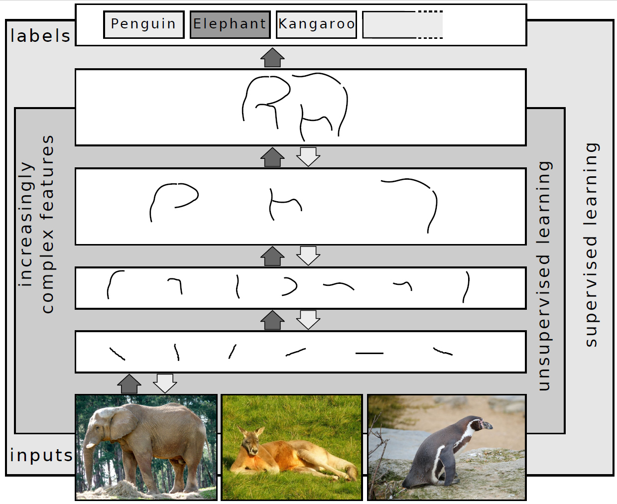
Fundamentally, deep learning refers to a class of machine learning algorithms in which a hierarchy of layers is used to transform input data into a progressively more abstract and composite representation. For example, in an image recognition model, the raw input may be an image (represented as a tensor of pixels). The first representational layer may attempt to identify basic shapes such as lines and circles, the second layer may compose and encode arrangements of edges, the third layer may encode a nose and eyes, and the fourth layer may recognize that the image contains a face.
Importantly, a deep learning process can learn which features to optimally place at which level on its own. Prior to deep learning, machine learning techniques often involved hand-crafted feature engineering to transform the data into a more suitable representation for a classification algorithm to operate on. In the deep learning approach, features are not hand-crafted and the model discovers useful feature representations from the data automatically. This does not eliminate the need for hand-tuning; for example, varying numbers of layers and layer sizes can provide different degrees of abstraction.[8][2]
The word "deep" in "deep learning" refers to the number of layers through which the data is transformed. More precisely, deep learning systems have a substantial credit assignment path (CAP) depth. The CAP is the chain of transformations from input to output. CAPs describe potentially causal connections between input and output. For a feedforward neural network, the depth of the CAPs is that of the network and is the number of hidden layers plus one (as the output layer is also parameterized). For recurrent neural networks, in which a signal may propagate through a layer more than once, the CAP depth is potentially unlimited.[9] No universally agreed-upon threshold of depth divides shallow learning from deep learning, but most researchers agree that deep learning involves CAP depth higher than two. CAP of depth two has been shown to be a universal approximator in the sense that it can emulate any function.[10] Beyond that, more layers do not add to the function approximator ability of the network. Deep models (CAP > two) are able to extract better features than shallow models and hence, extra layers help in learning the features effectively.
Deep learning architectures can be constructed with a greedy layer-by-layer method.[11] Deep learning helps to disentangle these abstractions and pick out which features improve performance.[8]
Deep learning algorithms can be applied to unsupervised learning tasks. This is an important benefit because unlabeled data is more abundant than the labeled data. Examples of deep structures that can be trained in an unsupervised manner are deep belief networks.[8][12]
The term deep learning was introduced to the machine learning community by Rina Dechter in 1986,[13] and to artificial neural networks by Igor Aizenberg and colleagues in 2000, in the context of Boolean threshold neurons.[14][15] Although the history of its appearance is apparently more complicated.[16]
Interpretations
[edit]Deep neural networks are generally interpreted in terms of the universal approximation theorem[17][18][19][20][21] or probabilistic inference.[22][23][8][9][24]
The classic universal approximation theorem concerns the capacity of feedforward neural networks with a single hidden layer of finite size to approximate continuous functions.[17][18][19][20] In 1989, the first proof was published by George Cybenko for sigmoid activation functions[17] and was generalised to feed-forward multi-layer architectures in 1991 by Kurt Hornik.[18] Recent work also showed that universal approximation also holds for non-bounded activation functions such as Kunihiko Fukushima's rectified linear unit.[25][26]
The universal approximation theorem for deep neural networks concerns the capacity of networks with bounded width but the depth is allowed to grow. Lu et al.[21] proved that if the width of a deep neural network with ReLU activation is strictly larger than the input dimension, then the network can approximate any Lebesgue integrable function; if the width is smaller or equal to the input dimension, then a deep neural network is not a universal approximator.
The probabilistic interpretation[24] derives from the field of machine learning. It features inference,[23][7][8][9][12][24] as well as the optimization concepts of training and testing, related to fitting and generalization, respectively. More specifically, the probabilistic interpretation considers the activation nonlinearity as a cumulative distribution function.[24] The probabilistic interpretation led to the introduction of dropout as regularizer in neural networks. The probabilistic interpretation was introduced by researchers including Hopfield, Widrow and Narendra and popularized in surveys such as the one by Bishop.[27]
History
[edit]Before 1980
[edit]There are two types of artificial neural network (ANN): feedforward neural network (FNN) or multilayer perceptron (MLP) and recurrent neural networks (RNN). RNNs have cycles in their connectivity structure, FNNs don't. In the 1920s, Wilhelm Lenz and Ernst Ising created the Ising model[28][29] which is essentially a non-learning RNN architecture consisting of neuron-like threshold elements. In 1972, Shun'ichi Amari made this architecture adaptive.[30][31] His learning RNN was republished by John Hopfield in 1982.[32] Other early recurrent neural networks were published by Kaoru Nakano in 1971.[33][34] Already in 1948, Alan Turing produced work on "Intelligent Machinery" that was not published in his lifetime,[35] containing "ideas related to artificial evolution and learning RNNs".[31]
Frank Rosenblatt (1958)[36] proposed the perceptron, an MLP with 3 layers: an input layer, a hidden layer with randomized weights that did not learn, and an output layer. He later published a 1962 book that also introduced variants and computer experiments, including a version with four-layer perceptrons "with adaptive preterminal networks" where the last two layers have learned weights (here he credits H. D. Block and B. W. Knight).[37]: section 16 The book cites an earlier network by R. D. Joseph (1960)[38] "functionally equivalent to a variation of" this four-layer system (the book mentions Joseph over 30 times). Should Joseph therefore be considered the originator of proper adaptive multilayer perceptrons with learning hidden units? Unfortunately, the learning algorithm was not a functional one, and fell into oblivion.
The first working deep learning algorithm was the Group method of data handling, a method to train arbitrarily deep neural networks, published by Alexey Ivakhnenko and Lapa in 1965. They regarded it as a form of polynomial regression,[39] or a generalization of Rosenblatt's perceptron to handle more complex, nonlinear, and hierarchical relationships.[40] A 1971 paper described a deep network with eight layers trained by this method,[41] which is based on layer by layer training through regression analysis. Superfluous hidden units are pruned using a separate validation set. Since the activation functions of the nodes are Kolmogorov-Gabor polynomials, these were also the first deep networks with multiplicative units or "gates".[31]
The first deep learning multilayer perceptron trained by stochastic gradient descent[42] was published in 1967 by Shun'ichi Amari.[43] In computer experiments conducted by Amari's student Saito, a five layer MLP with two modifiable layers learned internal representations to classify non-linearily separable pattern classes.[31] Subsequent developments in hardware and hyperparameter tunings have made end-to-end stochastic gradient descent the currently dominant training technique.
In 1969, Kunihiko Fukushima introduced the ReLU (rectified linear unit) activation function.[25][31] The rectifier has become the most popular activation function for deep learning.[44]
Deep learning architectures for convolutional neural networks (CNNs) with convolutional layers and downsampling layers began with the Neocognitron introduced by Kunihiko Fukushima in 1979, though not trained by backpropagation.[45][46]
Backpropagation is an efficient application of the chain rule derived by Gottfried Wilhelm Leibniz in 1673[47] to networks of differentiable nodes. The terminology "back-propagating errors" was actually introduced in 1962 by Rosenblatt,[37] but he did not know how to implement this, although Henry J. Kelley had a continuous precursor of backpropagation in 1960 in the context of control theory.[48] The modern form of backpropagation was first published in Seppo Linnainmaa's master thesis (1970).[49][50][31] G.M. Ostrovski et al. republished it in 1971.[51][52] Paul Werbos applied backpropagation to neural networks in 1982[53] (his 1974 PhD thesis, reprinted in a 1994 book,[54] did not yet describe the algorithm[52]). In 1986, David E. Rumelhart et al. popularised backpropagation but did not cite the original work.[55][56]
1980s-2000s
[edit]The time delay neural network (TDNN) was introduced in 1987 by Alex Waibel to apply CNN to phoneme recognition. It used convolutions, weight sharing, and backpropagation.[57][58] In 1988, Wei Zhang applied a backpropagation-trained CNN to alphabet recognition.[59] In 1989, Yann LeCun et al. created a CNN called LeNet for recognizing handwritten ZIP codes on mail. Training required 3 days.[60] In 1990, Wei Zhang implemented a CNN on optical computing hardware.[61] In 1991, a CNN was applied to medical image object segmentation[62] and breast cancer detection in mammograms.[63] LeNet-5 (1998), a 7-level CNN by Yann LeCun et al., that classifies digits, was applied by several banks to recognize hand-written numbers on checks digitized in 32x32 pixel images.[64]
Recurrent neural networks (RNN)[28][30] were further developed in the 1980s. Recurrence is used for sequence processing, and when a recurrent network is unrolled, it mathematically resembles a deep feedforward layer. Consequently, they have similar properties and issues, and their developments had mutual influences. In RNN, two early influential works were the Jordan network (1986)[65] and the Elman network (1990),[66] which applied RNN to study problems in cognitive psychology.
In the 1980s, backpropagation did not work well for deep learning with long credit assignment paths. To overcome this problem, in 1991, Jürgen Schmidhuber proposed a hierarchy of RNNs pre-trained one level at a time by self-supervised learning where each RNN tries to predict its own next input, which is the next unexpected input of the RNN below.[67][68] This "neural history compressor" uses predictive coding to learn internal representations at multiple self-organizing time scales. This can substantially facilitate downstream deep learning. The RNN hierarchy can be collapsed into a single RNN, by distilling a higher level chunker network into a lower level automatizer network.[67][68][31] In 1993, a neural history compressor solved a "Very Deep Learning" task that required more than 1000 subsequent layers in an RNN unfolded in time.[69] The "P" in ChatGPT refers to such pre-training.
Sepp Hochreiter's diploma thesis (1991)[70] implemented the neural history compressor,[67] and identified and analyzed the vanishing gradient problem.[70][71] Hochreiter proposed recurrent residual connections to solve the vanishing gradient problem. This led to the long short-term memory (LSTM), published in 1995.[72] LSTM can learn "very deep learning" tasks[9] with long credit assignment paths that require memories of events that happened thousands of discrete time steps before. That LSTM was not yet the modern architecture, which required a "forget gate", introduced in 1999,[73] which became the standard RNN architecture.
In 1991, Jürgen Schmidhuber also published adversarial neural networks that contest with each other in the form of a zero-sum game, where one network's gain is the other network's loss.[74][75] The first network is a generative model that models a probability distribution over output patterns. The second network learns by gradient descent to predict the reactions of the environment to these patterns. This was called "artificial curiosity". In 2014, this principle was used in generative adversarial networks (GANs).[76]
During 1985–1995, inspired by statistical mechanics, several architectures and methods were developed by Terry Sejnowski, Peter Dayan, Geoffrey Hinton, etc., including the Boltzmann machine,[77] restricted Boltzmann machine,[78] Helmholtz machine,[79] and the wake-sleep algorithm.[80] These were designed for unsupervised learning of deep generative models. However, those were more computationally expensive compared to backpropagation. Boltzmann machine learning algorithm, published in 1985, was briefly popular before being eclipsed by the backpropagation algorithm in 1986. (p. 112 [81]). A 1988 network became state of the art in protein structure prediction, an early application of deep learning to bioinformatics.[82]
Both shallow and deep learning (e.g., recurrent nets) of ANNs for speech recognition have been explored for many years.[83][84][85] These methods never outperformed non-uniform internal-handcrafting Gaussian mixture model/Hidden Markov model (GMM-HMM) technology based on generative models of speech trained discriminatively.[86] Key difficulties have been analyzed, including gradient diminishing[70] and weak temporal correlation structure in neural predictive models.[87][88] Additional difficulties were the lack of training data and limited computing power.
Most speech recognition researchers moved away from neural nets to pursue generative modeling. An exception was at SRI International in the late 1990s. Funded by the US government's NSA and DARPA, SRI researched in speech and speaker recognition. The speaker recognition team led by Larry Heck reported significant success with deep neural networks in speech processing in the 1998 NIST Speaker Recognition benchmark.[89][90] It was deployed in the Nuance Verifier, representing the first major industrial application of deep learning.[91]
The principle of elevating "raw" features over hand-crafted optimization was first explored successfully in the architecture of deep autoencoder on the "raw" spectrogram or linear filter-bank features in the late 1990s,[90] showing its superiority over the Mel-Cepstral features that contain stages of fixed transformation from spectrograms. The raw features of speech, waveforms, later produced excellent larger-scale results.[92]
2000s
[edit]Neural networks entered a lull, and simpler models that use task-specific handcrafted features such as Gabor filters and support vector machines (SVMs) became the preferred choices in the 1990s and 2000s, because of artificial neural networks' computational cost and a lack of understanding of how the brain wires its biological networks.[citation needed]
In 2003, LSTM became competitive with traditional speech recognizers on certain tasks.[93] In 2006, Alex Graves, Santiago Fernández, Faustino Gomez, and Schmidhuber combined it with connectionist temporal classification (CTC)[94] in stacks of LSTMs.[95] In 2009, it became the first RNN to win a pattern recognition contest, in connected handwriting recognition.[96][9]
In 2006, publications by Geoff Hinton, Ruslan Salakhutdinov, Osindero and Teh[97][98] deep belief networks were developed for generative modeling. They are trained by training one restricted Boltzmann machine, then freezing it and training another one on top of the first one, and so on, then optionally fine-tuned using supervised backpropagation.[99] They could model high-dimensional probability distributions, such as the distribution of MNIST images, but convergence was slow.[100][101][102]
The impact of deep learning in industry began in the early 2000s, when CNNs already processed an estimated 10% to 20% of all the checks written in the US, according to Yann LeCun.[103] Industrial applications of deep learning to large-scale speech recognition started around 2010.
The 2009 NIPS Workshop on Deep Learning for Speech Recognition was motivated by the limitations of deep generative models of speech, and the possibility that given more capable hardware and large-scale data sets that deep neural nets might become practical. It was believed that pre-training DNNs using generative models of deep belief nets (DBN) would overcome the main difficulties of neural nets. However, it was discovered that replacing pre-training with large amounts of training data for straightforward backpropagation when using DNNs with large, context-dependent output layers produced error rates dramatically lower than then-state-of-the-art Gaussian mixture model (GMM)/Hidden Markov Model (HMM) and also than more-advanced generative model-based systems.[104] The nature of the recognition errors produced by the two types of systems was characteristically different,[105] offering technical insights into how to integrate deep learning into the existing highly efficient, run-time speech decoding system deployed by all major speech recognition systems.[23][106][107] Analysis around 2009–2010, contrasting the GMM (and other generative speech models) vs. DNN models, stimulated early industrial investment in deep learning for speech recognition.[105] That analysis was done with comparable performance (less than 1.5% in error rate) between discriminative DNNs and generative models.[104][105][108] In 2010, researchers extended deep learning from TIMIT to large vocabulary speech recognition, by adopting large output layers of the DNN based on context-dependent HMM states constructed by decision trees.[109][110][111][106]
Deep learning revolution
[edit]
The deep learning revolution started around CNN- and GPU-based computer vision.
Although CNNs trained by backpropagation had been around for decades and GPU implementations of NNs for years,[112] including CNNs,[113] faster implementations of CNNs on GPUs were needed to progress on computer vision. Later, as deep learning becomes widespread, specialized hardware and algorithm optimizations were developed specifically for deep learning.[114]
A key advance for the deep learning revolution was hardware advances, especially GPU. Some early work dated back to 2004.[112][113] In 2009, Raina, Madhavan, and Andrew Ng reported a 100M deep belief network trained on 30 Nvidia GeForce GTX 280 GPUs, an early demonstration of GPU-based deep learning. They reported up to 70 times faster training.[115]
In 2011, a CNN named DanNet[116][117] by Dan Ciresan, Ueli Meier, Jonathan Masci, Luca Maria Gambardella, and Jürgen Schmidhuber achieved for the first time superhuman performance in a visual pattern recognition contest, outperforming traditional methods by a factor of 3.[9] It then won more contests.[118][119] They also showed how max-pooling CNNs on GPU improved performance significantly.[3]
In 2012, Andrew Ng and Jeff Dean created an FNN that learned to recognize higher-level concepts, such as cats, only from watching unlabeled images taken from YouTube videos.[120]
In October 2012, AlexNet by Alex Krizhevsky, Ilya Sutskever, and Geoffrey Hinton[4] won the large-scale ImageNet competition by a significant margin over shallow machine learning methods. Further incremental improvements included the VGG-16 network by Karen Simonyan and Andrew Zisserman[121] and Google's Inceptionv3.[122]
The success in image classification was then extended to the more challenging task of generating descriptions (captions) for images, often as a combination of CNNs and LSTMs.[123][124][125]
In 2014, the state of the art was training "very deep neural network" with 20 to 30 layers.[126] Stacking too many layers led to a steep reduction in training accuracy,[127] known as the "degradation" problem.[128] In 2015, two techniques were developed to train very deep networks: the highway network was published in May 2015, and the residual neural network (ResNet)[129] in Dec 2015. ResNet behaves like an open-gated Highway Net.
Around the same time, deep learning started impacting the field of art. Early examples included Google DeepDream (2015), and neural style transfer (2015),[130] both of which were based on pretrained image classification neural networks, such as VGG-19.
Generative adversarial network (GAN) by (Ian Goodfellow et al., 2014)[131] (based on Jürgen Schmidhuber's principle of artificial curiosity[74][76]) became state of the art in generative modeling during 2014-2018 period. Excellent image quality is achieved by Nvidia's StyleGAN (2018)[132] based on the Progressive GAN by Tero Karras et al.[133] Here the GAN generator is grown from small to large scale in a pyramidal fashion. Image generation by GAN reached popular success, and provoked discussions concerning deepfakes.[134] Diffusion models (2015)[135] eclipsed GANs in generative modeling since then, with systems such as DALL·E 2 (2022) and Stable Diffusion (2022).
In 2015, Google's speech recognition improved by 49% by an LSTM-based model, which they made available through Google Voice Search on smartphone.[136][137]
Deep learning is part of state-of-the-art systems in various disciplines, particularly computer vision and automatic speech recognition (ASR). Results on commonly used evaluation sets such as TIMIT (ASR) and MNIST (image classification), as well as a range of large-vocabulary speech recognition tasks have steadily improved.[104][138] Convolutional neural networks were superseded for ASR by LSTM.[137][139][140][141] but are more successful in computer vision.
Yoshua Bengio, Geoffrey Hinton and Yann LeCun were awarded the 2018 Turing Award for "conceptual and engineering breakthroughs that have made deep neural networks a critical component of computing".[142]
Neural networks
[edit]

In reality, textures and outlines would not be represented by single nodes, but rather by associated weight patterns of multiple nodes.
Artificial neural networks (ANNs) or connectionist systems are computing systems inspired by the biological neural networks that constitute animal brains. Such systems learn (progressively improve their ability) to do tasks by considering examples, generally without task-specific programming. For example, in image recognition, they might learn to identify images that contain cats by analyzing example images that have been manually labeled as "cat" or "no cat" and using the analytic results to identify cats in other images. They have found most use in applications difficult to express with a traditional computer algorithm using rule-based programming.
An ANN is based on a collection of connected units called artificial neurons, (analogous to biological neurons in a biological brain). Each connection (synapse) between neurons can transmit a signal to another neuron. The receiving (postsynaptic) neuron can process the signal(s) and then signal downstream neurons connected to it. Neurons may have state, generally represented by real numbers, typically between 0 and 1. Neurons and synapses may also have a weight that varies as learning proceeds, which can increase or decrease the strength of the signal that it sends downstream.
Typically, neurons are organized in layers. Different layers may perform different kinds of transformations on their inputs. Signals travel from the first (input), to the last (output) layer, possibly after traversing the layers multiple times.
The original goal of the neural network approach was to solve problems in the same way that a human brain would. Over time, attention focused on matching specific mental abilities, leading to deviations from biology such as backpropagation, or passing information in the reverse direction and adjusting the network to reflect that information.
Neural networks have been used on a variety of tasks, including computer vision, speech recognition, machine translation, social network filtering, playing board and video games and medical diagnosis.
As of 2017, neural networks typically have a few thousand to a few million units and millions of connections. Despite this number being several order of magnitude less than the number of neurons on a human brain, these networks can perform many tasks at a level beyond that of humans (e.g., recognizing faces, or playing "Go"[144]).
Deep neural networks
[edit]A deep neural network (DNN) is an artificial neural network with multiple layers between the input and output layers.[7][9] There are different types of neural networks but they always consist of the same components: neurons, synapses, weights, biases, and functions.[145] These components as a whole function in a way that mimics functions of the human brain, and can be trained like any other ML algorithm.[citation needed]
For example, a DNN that is trained to recognize dog breeds will go over the given image and calculate the probability that the dog in the image is a certain breed. The user can review the results and select which probabilities the network should display (above a certain threshold, etc.) and return the proposed label. Each mathematical manipulation as such is considered a layer,[146] and complex DNN have many layers, hence the name "deep" networks.
DNNs can model complex non-linear relationships. DNN architectures generate compositional models where the object is expressed as a layered composition of primitives.[147] The extra layers enable composition of features from lower layers, potentially modeling complex data with fewer units than a similarly performing shallow network.[7] For instance, it was proved that sparse multivariate polynomials are exponentially easier to approximate with DNNs than with shallow networks.[148]
Deep architectures include many variants of a few basic approaches. Each architecture has found success in specific domains. It is not always possible to compare the performance of multiple architectures, unless they have been evaluated on the same data sets.[146]
DNNs are typically feedforward networks in which data flows from the input layer to the output layer without looping back. At first, the DNN creates a map of virtual neurons and assigns random numerical values, or "weights", to connections between them. The weights and inputs are multiplied and return an output between 0 and 1. If the network did not accurately recognize a particular pattern, an algorithm would adjust the weights.[149] That way the algorithm can make certain parameters more influential, until it determines the correct mathematical manipulation to fully process the data.
Recurrent neural networks, in which data can flow in any direction, are used for applications such as language modeling.[150][151][152][153][154] Long short-term memory is particularly effective for this use.[155][156]
Convolutional neural networks (CNNs) are used in computer vision.[157] CNNs also have been applied to acoustic modeling for automatic speech recognition (ASR).[158]
Challenges
[edit]As with ANNs, many issues can arise with naively trained DNNs. Two common issues are overfitting and computation time.
DNNs are prone to overfitting because of the added layers of abstraction, which allow them to model rare dependencies in the training data. Regularization methods such as Ivakhnenko's unit pruning[41] or weight decay (-regularization) or sparsity (-regularization) can be applied during training to combat overfitting.[159] Alternatively dropout regularization randomly omits units from the hidden layers during training. This helps to exclude rare dependencies.[160] Another interesting recent development is research into models of just enough complexity through an estimation of the intrinsic complexity of the task being modelled. This approach has been successfully applied for multivariate time series prediction tasks such as traffic prediction.[161] Finally, data can be augmented via methods such as cropping and rotating such that smaller training sets can be increased in size to reduce the chances of overfitting.[162]


DNNs must consider many training parameters, such as the size (number of layers and number of units per layer), the learning rate, and initial weights. Sweeping through the parameter space for optimal parameters may not be feasible due to the cost in time and computational resources. Various tricks, such as batching (computing the gradient on several training examples at once rather than individual examples)[163] speed up computation. Large processing capabilities of many-core architectures (such as GPUs or the Intel Xeon Phi) have produced significant speedups in training, because of the suitability of such processing architectures for the matrix and vector computations.[164][165]
Alternatively, engineers may look for other types of neural networks with more straightforward and convergent training algorithms. CMAC (cerebellar model articulation controller) is one such kind of neural network. It doesn't require learning rates or randomized initial weights. The training process can be guaranteed to converge in one step with a new batch of data, and the computational complexity of the training algorithm is linear with respect to the number of neurons involved.[166][167]
Hardware
[edit]Since the 2010s, advances in both machine learning algorithms and computer hardware have led to more efficient methods for training deep neural networks that contain many layers of non-linear hidden units and a very large output layer.[168] By 2019, graphics processing units (GPUs), often with AI-specific enhancements, had displaced CPUs as the dominant method for training large-scale commercial cloud AI .[169] OpenAI estimated the hardware computation used in the largest deep learning projects from AlexNet (2012) to AlphaZero (2017) and found a 300,000-fold increase in the amount of computation required, with a doubling-time trendline of 3.4 months.[170][171]
Special electronic circuits called deep learning processors were designed to speed up deep learning algorithms. Deep learning processors include neural processing units (NPUs) in Huawei cellphones[172] and cloud computing servers such as tensor processing units (TPU) in the Google Cloud Platform.[173] Cerebras Systems has also built a dedicated system to handle large deep learning models, the CS-2, based on the largest processor in the industry, the second-generation Wafer Scale Engine (WSE-2).[174][175]
Atomically thin semiconductors are considered promising for energy-efficient deep learning hardware where the same basic device structure is used for both logic operations and data storage. In 2020, Marega et al. published experiments with a large-area active channel material for developing logic-in-memory devices and circuits based on floating-gate field-effect transistors (FGFETs).[176]
In 2021, J. Feldmann et al. proposed an integrated photonic hardware accelerator for parallel convolutional processing.[177] The authors identify two key advantages of integrated photonics over its electronic counterparts: (1) massively parallel data transfer through wavelength division multiplexing in conjunction with frequency combs, and (2) extremely high data modulation speeds.[177] Their system can execute trillions of multiply-accumulate operations per second, indicating the potential of integrated photonics in data-heavy AI applications.[177]
Applications
[edit]Automatic speech recognition
[edit]Large-scale automatic speech recognition is the first and most convincing successful case of deep learning. LSTM RNNs can learn "Very Deep Learning" tasks[9] that involve multi-second intervals containing speech events separated by thousands of discrete time steps, where one time step corresponds to about 10 ms. LSTM with forget gates[156] is competitive with traditional speech recognizers on certain tasks.[93]
The initial success in speech recognition was based on small-scale recognition tasks based on TIMIT. The data set contains 630 speakers from eight major dialects of American English, where each speaker reads 10 sentences.[178] Its small size lets many configurations be tried. More importantly, the TIMIT task concerns phone-sequence recognition, which, unlike word-sequence recognition, allows weak phone bigram language models. This lets the strength of the acoustic modeling aspects of speech recognition be more easily analyzed. The error rates listed below, including these early results and measured as percent phone error rates (PER), have been summarized since 1991.
| Method | Percent phone error rate (PER) (%) |
|---|---|
| Randomly Initialized RNN[179] | 26.1 |
| Bayesian Triphone GMM-HMM | 25.6 |
| Hidden Trajectory (Generative) Model | 24.8 |
| Monophone Randomly Initialized DNN | 23.4 |
| Monophone DBN-DNN | 22.4 |
| Triphone GMM-HMM with BMMI Training | 21.7 |
| Monophone DBN-DNN on fbank | 20.7 |
| Convolutional DNN[180] | 20.0 |
| Convolutional DNN w. Heterogeneous Pooling | 18.7 |
| Ensemble DNN/CNN/RNN[181] | 18.3 |
| Bidirectional LSTM | 17.8 |
| Hierarchical Convolutional Deep Maxout Network[182] | 16.5 |
The debut of DNNs for speaker recognition in the late 1990s and speech recognition around 2009-2011 and of LSTM around 2003–2007, accelerated progress in eight major areas:[23][108][106]
- Scale-up/out and accelerated DNN training and decoding
- Sequence discriminative training
- Feature processing by deep models with solid understanding of the underlying mechanisms
- Adaptation of DNNs and related deep models
- Multi-task and transfer learning by DNNs and related deep models
- CNNs and how to design them to best exploit domain knowledge of speech
- RNN and its rich LSTM variants
- Other types of deep models including tensor-based models and integrated deep generative/discriminative models.
More recent speech recognition models use Transformers or Temporal Convolution Networks with significant success and widespread applications.[183][184][185] All major commercial speech recognition systems (e.g., Microsoft Cortana, Xbox, Skype Translator, Amazon Alexa, Google Now, Apple Siri, Baidu and iFlyTek voice search, and a range of Nuance speech products, etc.) are based on deep learning.[23][186][187]
Image recognition
[edit]A common evaluation set for image classification is the MNIST database data set. MNIST is composed of handwritten digits and includes 60,000 training examples and 10,000 test examples. As with TIMIT, its small size lets users test multiple configurations. A comprehensive list of results on this set is available.[188]
Deep learning-based image recognition has become "superhuman", producing more accurate results than human contestants. This first occurred in 2011 in recognition of traffic signs, and in 2014, with recognition of human faces.[189][190]
Deep learning-trained vehicles now interpret 360° camera views.[191] Another example is Facial Dysmorphology Novel Analysis (FDNA) used to analyze cases of human malformation connected to a large database of genetic syndromes.
Visual art processing
[edit]Closely related to the progress that has been made in image recognition is the increasing application of deep learning techniques to various visual art tasks. DNNs have proven themselves capable, for example, of
- identifying the style period of a given painting[192][193]
- Neural Style Transfer – capturing the style of a given artwork and applying it in a visually pleasing manner to an arbitrary photograph or video[192][193]
- generating striking imagery based on random visual input fields.[192][193]
Natural language processing
[edit]Neural networks have been used for implementing language models since the early 2000s.[150] LSTM helped to improve machine translation and language modeling.[151][152][153]
Other key techniques in this field are negative sampling[194] and word embedding. Word embedding, such as word2vec, can be thought of as a representational layer in a deep learning architecture that transforms an atomic word into a positional representation of the word relative to other words in the dataset; the position is represented as a point in a vector space. Using word embedding as an RNN input layer allows the network to parse sentences and phrases using an effective compositional vector grammar. A compositional vector grammar can be thought of as probabilistic context free grammar (PCFG) implemented by an RNN.[195] Recursive auto-encoders built atop word embeddings can assess sentence similarity and detect paraphrasing.[195] Deep neural architectures provide the best results for constituency parsing,[196] sentiment analysis,[197] information retrieval,[198][199] spoken language understanding,[200] machine translation,[151][201] contextual entity linking,[201] writing style recognition,[202] named-entity recognition (token classification),[203] text classification, and others.[204]
Recent developments generalize word embedding to sentence embedding.
Google Translate (GT) uses a large end-to-end long short-term memory (LSTM) network.[205][206][207][208] Google Neural Machine Translation (GNMT) uses an example-based machine translation method in which the system "learns from millions of examples".[206] It translates "whole sentences at a time, rather than pieces". Google Translate supports over one hundred languages.[206] The network encodes the "semantics of the sentence rather than simply memorizing phrase-to-phrase translations".[206][209] GT uses English as an intermediate between most language pairs.[209]
Drug discovery and toxicology
[edit]A large percentage of candidate drugs fail to win regulatory approval. These failures are caused by insufficient efficacy (on-target effect), undesired interactions (off-target effects), or unanticipated toxic effects.[210][211] Research has explored use of deep learning to predict the biomolecular targets,[212][213] off-targets, and toxic effects of environmental chemicals in nutrients, household products and drugs.[214][215][216]
AtomNet is a deep learning system for structure-based rational drug design.[217] AtomNet was used to predict novel candidate biomolecules for disease targets such as the Ebola virus[218] and multiple sclerosis.[219][218]
In 2017 graph neural networks were used for the first time to predict various properties of molecules in a large toxicology data set.[220] In 2019, generative neural networks were used to produce molecules that were validated experimentally all the way into mice.[221][222]
Recommendation systems
[edit]Recommendation systems have used deep learning to extract meaningful features for a latent factor model for content-based music and journal recommendations.[223][224] Multi-view deep learning has been applied for learning user preferences from multiple domains.[225] The model uses a hybrid collaborative and content-based approach and enhances recommendations in multiple tasks.
Bioinformatics
[edit]An autoencoder ANN was used in bioinformatics, to predict gene ontology annotations and gene-function relationships.[226]
In medical informatics, deep learning was used to predict sleep quality based on data from wearables[227] and predictions of health complications from electronic health record data.[228]
Deep neural networks have shown unparalleled performance in predicting protein structure, according to the sequence of the amino acids that make it up. In 2020, AlphaFold, a deep-learning based system, achieved a level of accuracy significantly higher than all previous computational methods.[229][230]
Deep Neural Network Estimations
[edit]Deep neural networks can be used to estimate the entropy of a stochastic process through an arrangement called a Neural Joint Entropy Estimator (NJEE).[231] Such an estimation provides insights on the effects of input random variables on an independent random variable. Practically, the DNN is trained as a classifier that maps an input vector or matrix X to an output probability distribution over the possible classes of random variable Y, given input X. For example, in image classification tasks, the NJEE maps a vector of pixels' color values to probabilities over possible image classes. In practice, the probability distribution of Y is obtained by a Softmax layer with number of nodes that is equal to the alphabet size of Y. NJEE uses continuously differentiable activation functions, such that the conditions for the universal approximation theorem holds. It is shown that this method provides a strongly consistent estimator and outperforms other methods in cases of large alphabet sizes.[231]
Medical image analysis
[edit]Deep learning has been shown to produce competitive results in medical applications such as cancer cell classification, lesion detection, organ segmentation and image enhancement.[232][233] Modern deep learning tools demonstrate the high accuracy of detecting various diseases and the helpfulness of their use by specialists to improve the diagnosis efficiency.[234][235]
Mobile advertising
[edit]Finding the appropriate mobile audience for mobile advertising is always challenging, since many data points must be considered and analyzed before a target segment can be created and used in ad serving by any ad server.[236] Deep learning has been used to interpret large, many-dimensioned advertising datasets. Many data points are collected during the request/serve/click internet advertising cycle. This information can form the basis of machine learning to improve ad selection.
Image restoration
[edit]Deep learning has been successfully applied to inverse problems such as denoising, super-resolution, inpainting, and film colorization.[237] These applications include learning methods such as "Shrinkage Fields for Effective Image Restoration"[238] which trains on an image dataset, and Deep Image Prior, which trains on the image that needs restoration.
Financial fraud detection
[edit]Deep learning is being successfully applied to financial fraud detection, tax evasion detection,[239] and anti-money laundering.[240]
Materials science
[edit]In November 2023, researchers at Google DeepMind and Lawrence Berkeley National Laboratory announced that they had developed an AI system known as GNoME. This system has contributed to materials science by discovering over 2 million new materials within a relatively short timeframe. GNoME employs deep learning techniques to efficiently explore potential material structures, achieving a significant increase in the identification of stable inorganic crystal structures. The system's predictions were validated through autonomous robotic experiments, demonstrating a noteworthy success rate of 71%. The data of newly discovered materials is publicly available through the Materials Project database, offering researchers the opportunity to identify materials with desired properties for various applications. This development has implications for the future of scientific discovery and the integration of AI in material science research, potentially expediting material innovation and reducing costs in product development. The use of AI and deep learning suggests the possibility of minimizing or eliminating manual lab experiments and allowing scientists to focus more on the design and analysis of unique compounds.[241][242][243]
Military
[edit]The United States Department of Defense applied deep learning to train robots in new tasks through observation.[244]
Partial differential equations
[edit]Physics informed neural networks have been used to solve partial differential equations in both forward and inverse problems in a data driven manner.[245] One example is the reconstructing fluid flow governed by the Navier-Stokes equations. Using physics informed neural networks does not require the often expensive mesh generation that conventional CFD methods rely on.[246][247]. It is evident that geometric and physical constraints have a synergistic effect on neural PDE surrogates, thereby enhancing their efficacy in predicting stable and super long rollouts.[248]
Deep backward stochastic differential equation method
[edit]Deep backward stochastic differential equation method is a numerical method that combines deep learning with Backward stochastic differential equation (BSDE). This method is particularly useful for solving high-dimensional problems in financial mathematics. By leveraging the powerful function approximation capabilities of deep neural networks, deep BSDE addresses the computational challenges faced by traditional numerical methods in high-dimensional settings. Specifically, traditional methods like finite difference methods or Monte Carlo simulations often struggle with the curse of dimensionality, where computational cost increases exponentially with the number of dimensions. Deep BSDE methods, however, employ deep neural networks to approximate solutions of high-dimensional partial differential equations (PDEs), effectively reducing the computational burden.[249]
In addition, the integration of Physics-informed neural networks (PINNs) into the deep BSDE framework enhances its capability by embedding the underlying physical laws directly into the neural network architecture. This ensures that the solutions not only fit the data but also adhere to the governing stochastic differential equations. PINNs leverage the power of deep learning while respecting the constraints imposed by the physical models, resulting in more accurate and reliable solutions for financial mathematics problems.
Image reconstruction
[edit]Image reconstruction is the reconstruction of the underlying images from the image-related measurements. Several works showed the better and superior performance of the deep learning methods compared to analytical methods for various applications, e.g., spectral imaging [250] and ultrasound imaging.[251]
Weather prediction
[edit]Traditional weather prediction systems solve a very complex system of partial differential equations. GraphCast is a deep learning based model, trained on a long history of weather data to predict how weather patterns change over time. It is able to predict weather conditions for up to 10 days globally, at a very detailed level, and in under a minute, with precision similar to state of the art systems.[252][253]
Epigenetic clock
[edit]An epigenetic clock is a biochemical test that can be used to measure age. Galkin et al. used deep neural networks to train an epigenetic aging clock of unprecedented accuracy using >6,000 blood samples.[254] The clock uses information from 1000 CpG sites and predicts people with certain conditions older than healthy controls: IBD, frontotemporal dementia, ovarian cancer, obesity. The aging clock was planned to be released for public use in 2021 by an Insilico Medicine spinoff company Deep Longevity.
Relation to human cognitive and brain development
[edit]Deep learning is closely related to a class of theories of brain development (specifically, neocortical development) proposed by cognitive neuroscientists in the early 1990s.[255][256][257][258] These developmental theories were instantiated in computational models, making them predecessors of deep learning systems. These developmental models share the property that various proposed learning dynamics in the brain (e.g., a wave of nerve growth factor) support the self-organization somewhat analogous to the neural networks utilized in deep learning models. Like the neocortex, neural networks employ a hierarchy of layered filters in which each layer considers information from a prior layer (or the operating environment), and then passes its output (and possibly the original input), to other layers. This process yields a self-organizing stack of transducers, well-tuned to their operating environment. A 1995 description stated, "...the infant's brain seems to organize itself under the influence of waves of so-called trophic-factors ... different regions of the brain become connected sequentially, with one layer of tissue maturing before another and so on until the whole brain is mature".[259]
A variety of approaches have been used to investigate the plausibility of deep learning models from a neurobiological perspective. On the one hand, several variants of the backpropagation algorithm have been proposed in order to increase its processing realism.[260][261] Other researchers have argued that unsupervised forms of deep learning, such as those based on hierarchical generative models and deep belief networks, may be closer to biological reality.[262][263] In this respect, generative neural network models have been related to neurobiological evidence about sampling-based processing in the cerebral cortex.[264]
Although a systematic comparison between the human brain organization and the neuronal encoding in deep networks has not yet been established, several analogies have been reported. For example, the computations performed by deep learning units could be similar to those of actual neurons[265] and neural populations.[266] Similarly, the representations developed by deep learning models are similar to those measured in the primate visual system[267] both at the single-unit[268] and at the population[269] levels.
Commercial activity
[edit]Facebook's AI lab performs tasks such as automatically tagging uploaded pictures with the names of the people in them.[270]
Google's DeepMind Technologies developed a system capable of learning how to play Atari video games using only pixels as data input. In 2015 they demonstrated their AlphaGo system, which learned the game of Go well enough to beat a professional Go player.[271][272][273] Google Translate uses a neural network to translate between more than 100 languages.
In 2017, Covariant.ai was launched, which focuses on integrating deep learning into factories.[274]
As of 2008,[275] researchers at The University of Texas at Austin (UT) developed a machine learning framework called Training an Agent Manually via Evaluative Reinforcement, or TAMER, which proposed new methods for robots or computer programs to learn how to perform tasks by interacting with a human instructor.[244] First developed as TAMER, a new algorithm called Deep TAMER was later introduced in 2018 during a collaboration between U.S. Army Research Laboratory (ARL) and UT researchers. Deep TAMER used deep learning to provide a robot with the ability to learn new tasks through observation.[244] Using Deep TAMER, a robot learned a task with a human trainer, watching video streams or observing a human perform a task in-person. The robot later practiced the task with the help of some coaching from the trainer, who provided feedback such as "good job" and "bad job".[276]
Criticism and comment
[edit]Deep learning has attracted both criticism and comment, in some cases from outside the field of computer science.
Theory
[edit]A main criticism concerns the lack of theory surrounding some methods.[277] Learning in the most common deep architectures is implemented using well-understood gradient descent. However, the theory surrounding other algorithms, such as contrastive divergence is less clear.[citation needed] (e.g., Does it converge? If so, how fast? What is it approximating?) Deep learning methods are often looked at as a black box, with most confirmations done empirically, rather than theoretically.[278]
In further reference to the idea that artistic sensitivity might be inherent in relatively low levels of the cognitive hierarchy, a published series of graphic representations of the internal states of deep (20-30 layers) neural networks attempting to discern within essentially random data the images on which they were trained[279] demonstrate a visual appeal: the original research notice received well over 1,000 comments, and was the subject of what was for a time the most frequently accessed article on The Guardian's[280] website.
With the support of Innovation Diffusion Theory (IDT), a study analyzed the diffusion of Deep Learning[281] in BRICS and OECD countries using data from Google Trends.
Errors
[edit]Some deep learning architectures display problematic behaviors,[282] such as confidently classifying unrecognizable images as belonging to a familiar category of ordinary images (2014)[283] and misclassifying minuscule perturbations of correctly classified images (2013).[284] Goertzel hypothesized that these behaviors are due to limitations in their internal representations and that these limitations would inhibit integration into heterogeneous multi-component artificial general intelligence (AGI) architectures.[282] These issues may possibly be addressed by deep learning architectures that internally form states homologous to image-grammar[285] decompositions of observed entities and events.[282] Learning a grammar (visual or linguistic) from training data would be equivalent to restricting the system to commonsense reasoning that operates on concepts in terms of grammatical production rules and is a basic goal of both human language acquisition[286] and artificial intelligence (AI).[287]
Cyber threat
[edit]As deep learning moves from the lab into the world, research and experience show that artificial neural networks are vulnerable to hacks and deception.[288] By identifying patterns that these systems use to function, attackers can modify inputs to ANNs in such a way that the ANN finds a match that human observers would not recognize. For example, an attacker can make subtle changes to an image such that the ANN finds a match even though the image looks to a human nothing like the search target. Such manipulation is termed an "adversarial attack".[289]
In 2016 researchers used one ANN to doctor images in trial and error fashion, identify another's focal points, and thereby generate images that deceived it. The modified images looked no different to human eyes. Another group showed that printouts of doctored images then photographed successfully tricked an image classification system.[290] One defense is reverse image search, in which a possible fake image is submitted to a site such as TinEye that can then find other instances of it. A refinement is to search using only parts of the image, to identify images from which that piece may have been taken.[291]
Another group showed that certain psychedelic spectacles could fool a facial recognition system into thinking ordinary people were celebrities, potentially allowing one person to impersonate another. In 2017 researchers added stickers to stop signs and caused an ANN to misclassify them.[290]
ANNs can however be further trained to detect attempts at deception, potentially leading attackers and defenders into an arms race similar to the kind that already defines the malware defense industry. ANNs have been trained to defeat ANN-based anti-malware software by repeatedly attacking a defense with malware that was continually altered by a genetic algorithm until it tricked the anti-malware while retaining its ability to damage the target.[290]
In 2016, another group demonstrated that certain sounds could make the Google Now voice command system open a particular web address, and hypothesized that this could "serve as a stepping stone for further attacks (e.g., opening a web page hosting drive-by malware)".[290]
In "data poisoning", false data is continually smuggled into a machine learning system's training set to prevent it from achieving mastery.[290]
Data collection ethics
[edit]The deep learning systems that are trained using supervised learning often rely on data that is created or annotated by humans, or both.[292] It has been argued that not only low-paid clickwork (such as on Amazon Mechanical Turk) is regularly deployed for this purpose, but also implicit forms of human microwork that are often not recognized as such.[293] The philosopher Rainer Mühlhoff distinguishes five types of "machinic capture" of human microwork to generate training data: (1) gamification (the embedding of annotation or computation tasks in the flow of a game), (2) "trapping and tracking" (e.g. CAPTCHAs for image recognition or click-tracking on Google search results pages), (3) exploitation of social motivations (e.g. tagging faces on Facebook to obtain labeled facial images), (4) information mining (e.g. by leveraging quantified-self devices such as activity trackers) and (5) clickwork.[293]
See also
[edit]- Applications of artificial intelligence
- Comparison of deep learning software
- Compressed sensing
- Differentiable programming
- Echo state network
- List of artificial intelligence projects
- Liquid state machine
- List of datasets for machine-learning research
- Reservoir computing
- Scale space and deep learning
- Sparse coding
- Stochastic parrot
- Topological deep learning
References
[edit]- ^ Schulz, Hannes; Behnke, Sven (1 November 2012). "Deep Learning". KI - Künstliche Intelligenz. 26 (4): 357–363. doi:10.1007/s13218-012-0198-z. ISSN 1610-1987. S2CID 220523562.
- ^ a b LeCun, Yann; Bengio, Yoshua; Hinton, Geoffrey (2015). "Deep Learning" (PDF). Nature. 521 (7553): 436–444. Bibcode:2015Natur.521..436L. doi:10.1038/nature14539. PMID 26017442. S2CID 3074096.
- ^ a b Ciresan, D.; Meier, U.; Schmidhuber, J. (2012). "Multi-column deep neural networks for image classification". 2012 IEEE Conference on Computer Vision and Pattern Recognition. pp. 3642–3649. arXiv:1202.2745. doi:10.1109/cvpr.2012.6248110. ISBN 978-1-4673-1228-8. S2CID 2161592.
- ^ a b Krizhevsky, Alex; Sutskever, Ilya; Hinton, Geoffrey (2012). "ImageNet Classification with Deep Convolutional Neural Networks" (PDF). NIPS 2012: Neural Information Processing Systems, Lake Tahoe, Nevada. Archived (PDF) from the original on 2017-01-10. Retrieved 2017-05-24.
- ^ "Google's AlphaGo AI wins three-match series against the world's best Go player". TechCrunch. 25 May 2017. Archived from the original on 17 June 2018. Retrieved 17 June 2018.
- ^ "Study urges caution when comparing neural networks to the brain". MIT News | Massachusetts Institute of Technology. 2022-11-02. Retrieved 2023-12-06.
- ^ a b c d Bengio, Yoshua (2009). "Learning Deep Architectures for AI" (PDF). Foundations and Trends in Machine Learning. 2 (1): 1–127. CiteSeerX 10.1.1.701.9550. doi:10.1561/2200000006. S2CID 207178999. Archived from the original (PDF) on 4 March 2016. Retrieved 3 September 2015.
- ^ a b c d e Bengio, Y.; Courville, A.; Vincent, P. (2013). "Representation Learning: A Review and New Perspectives". IEEE Transactions on Pattern Analysis and Machine Intelligence. 35 (8): 1798–1828. arXiv:1206.5538. Bibcode:2013ITPAM..35.1798B. doi:10.1109/tpami.2013.50. PMID 23787338. S2CID 393948.
- ^ a b c d e f g h Schmidhuber, J. (2015). "Deep Learning in Neural Networks: An Overview". Neural Networks. 61: 85–117. arXiv:1404.7828. doi:10.1016/j.neunet.2014.09.003. PMID 25462637. S2CID 11715509.
- ^ Shigeki, Sugiyama (12 April 2019). Human Behavior and Another Kind in Consciousness: Emerging Research and Opportunities: Emerging Research and Opportunities. IGI Global. ISBN 978-1-5225-8218-2.
- ^ Bengio, Yoshua; Lamblin, Pascal; Popovici, Dan; Larochelle, Hugo (2007). Greedy layer-wise training of deep networks (PDF). Advances in neural information processing systems. pp. 153–160. Archived (PDF) from the original on 2019-10-20. Retrieved 2019-10-06.
- ^ a b Hinton, G.E. (2009). "Deep belief networks". Scholarpedia. 4 (5): 5947. Bibcode:2009SchpJ...4.5947H. doi:10.4249/scholarpedia.5947.
- ^ Rina Dechter (1986). Learning while searching in constraint-satisfaction problems. University of California, Computer Science Department, Cognitive Systems Laboratory.Online Archived 2016-04-19 at the Wayback Machine
- ^ Aizenberg, I.N.; Aizenberg, N.N.; Vandewalle, J. (2000). Multi-Valued and Universal Binary Neurons. Science & Business Media. doi:10.1007/978-1-4757-3115-6. ISBN 978-0-7923-7824-2. Retrieved 27 December 2023.
- ^ Co-evolving recurrent neurons learn deep memory POMDPs. Proc. GECCO, Washington, D. C., pp. 1795–1802, ACM Press, New York, NY, USA, 2005.
- ^ Fradkov, Alexander L. (2020-01-01). "Early History of Machine Learning". IFAC-PapersOnLine. 21st IFAC World Congress. 53 (2): 1385–1390. doi:10.1016/j.ifacol.2020.12.1888. ISSN 2405-8963. S2CID 235081987.
- ^ a b c Cybenko (1989). "Approximations by superpositions of sigmoidal functions" (PDF). Mathematics of Control, Signals, and Systems. 2 (4): 303–314. Bibcode:1989MCSS....2..303C. doi:10.1007/bf02551274. S2CID 3958369. Archived from the original (PDF) on 10 October 2015.
- ^ a b c Hornik, Kurt (1991). "Approximation Capabilities of Multilayer Feedforward Networks". Neural Networks. 4 (2): 251–257. doi:10.1016/0893-6080(91)90009-t. S2CID 7343126.
- ^ a b Haykin, Simon S. (1999). Neural Networks: A Comprehensive Foundation. Prentice Hall. ISBN 978-0-13-273350-2.
- ^ a b Hassoun, Mohamad H. (1995). Fundamentals of Artificial Neural Networks. MIT Press. p. 48. ISBN 978-0-262-08239-6.
- ^ a b Lu, Z., Pu, H., Wang, F., Hu, Z., & Wang, L. (2017). The Expressive Power of Neural Networks: A View from the Width Archived 2019-02-13 at the Wayback Machine. Neural Information Processing Systems, 6231-6239.
- ^ Orhan, A. E.; Ma, W. J. (2017). "Efficient probabilistic inference in generic neural networks trained with non-probabilistic feedback". Nature Communications. 8 (1): 138. Bibcode:2017NatCo...8..138O. doi:10.1038/s41467-017-00181-8. PMC 5527101. PMID 28743932.
- ^ a b c d e Deng, L.; Yu, D. (2014). "Deep Learning: Methods and Applications" (PDF). Foundations and Trends in Signal Processing. 7 (3–4): 1–199. doi:10.1561/2000000039. Archived (PDF) from the original on 2016-03-14. Retrieved 2014-10-18.
- ^ a b c d Murphy, Kevin P. (24 August 2012). Machine Learning: A Probabilistic Perspective. MIT Press. ISBN 978-0-262-01802-9.
- ^ a b Fukushima, K. (1969). "Visual feature extraction by a multilayered network of analog threshold elements". IEEE Transactions on Systems Science and Cybernetics. 5 (4): 322–333. doi:10.1109/TSSC.1969.300225.
- ^ Sonoda, Sho; Murata, Noboru (2017). "Neural network with unbounded activation functions is universal approximator". Applied and Computational Harmonic Analysis. 43 (2): 233–268. arXiv:1505.03654. doi:10.1016/j.acha.2015.12.005. S2CID 12149203.
- ^ Bishop, Christopher M. (2006). Pattern Recognition and Machine Learning (PDF). Springer. ISBN 978-0-387-31073-2. Archived (PDF) from the original on 2017-01-11. Retrieved 2017-08-06.
- ^ a b "bibliotheca Augustana". www.hs-augsburg.de.
- ^ Brush, Stephen G. (1967). "History of the Lenz-Ising Model". Reviews of Modern Physics. 39 (4): 883–893. Bibcode:1967RvMP...39..883B. doi:10.1103/RevModPhys.39.883.
- ^ a b Amari, Shun-Ichi (1972). "Learning patterns and pattern sequences by self-organizing nets of threshold elements". IEEE Transactions. C (21): 1197–1206.
- ^ a b c d e f g Schmidhuber, Jürgen (2022). "Annotated History of Modern AI and Deep Learning". arXiv:2212.11279 [cs.NE].
- ^ Hopfield, J. J. (1982). "Neural networks and physical systems with emergent collective computational abilities". Proceedings of the National Academy of Sciences. 79 (8): 2554–2558. Bibcode:1982PNAS...79.2554H. doi:10.1073/pnas.79.8.2554. PMC 346238. PMID 6953413.
- ^ Nakano, Kaoru (1971). "Learning Process in a Model of Associative Memory". Pattern Recognition and Machine Learning. pp. 172–186. doi:10.1007/978-1-4615-7566-5_15. ISBN 978-1-4615-7568-9.
- ^ Nakano, Kaoru (1972). "Associatron-A Model of Associative Memory". IEEE Transactions on Systems, Man, and Cybernetics. SMC-2 (3): 380–388. doi:10.1109/TSMC.1972.4309133.
- ^ Turing, Alan (1992) [1948]. "Intelligent Machinery". In Ince, D.C. (ed.). Collected Works of AM Turing: Mechanical Intelligence. Vol. 1. Elsevier Science Publishers. p. 107. ISBN 0-444-88058-5.
- ^ Rosenblatt, F. (1958). "The perceptron: A probabilistic model for information storage and organization in the brain". Psychological Review. 65 (6): 386–408. doi:10.1037/h0042519. ISSN 1939-1471. PMID 13602029.
- ^ a b Rosenblatt, Frank (1962). Principles of Neurodynamics. Spartan, New York.
- ^ Joseph, R. D. (1960). Contributions to Perceptron Theory, Cornell Aeronautical Laboratory Report No. VG-11 96--G-7, Buffalo.
- ^ Ivakhnenko, A. G.; Lapa, V. G. (1967). Cybernetics and Forecasting Techniques. American Elsevier Publishing Co. ISBN 978-0-444-00020-0.
- ^ Ivakhnenko, A.G. (March 1970). "Heuristic self-organization in problems of engineering cybernetics". Automatica. 6 (2): 207–219. doi:10.1016/0005-1098(70)90092-0.
- ^ a b Ivakhnenko, Alexey (1971). "Polynomial theory of complex systems" (PDF). IEEE Transactions on Systems, Man, and Cybernetics. SMC-1 (4): 364–378. doi:10.1109/TSMC.1971.4308320. Archived (PDF) from the original on 2017-08-29. Retrieved 2019-11-05.
- ^ Robbins, H.; Monro, S. (1951). "A Stochastic Approximation Method". The Annals of Mathematical Statistics. 22 (3): 400. doi:10.1214/aoms/1177729586.
- ^ Amari, Shun'ichi (1967). "A theory of adaptive pattern classifier". IEEE Transactions. EC (16): 279–307.
- ^ Ramachandran, Prajit; Barret, Zoph; Quoc, V. Le (October 16, 2017). "Searching for Activation Functions". arXiv:1710.05941 [cs.NE].
- ^ Fukushima, K. (1979). "Neural network model for a mechanism of pattern recognition unaffected by shift in position—Neocognitron". Trans. IECE (In Japanese). J62-A (10): 658–665. doi:10.1007/bf00344251. PMID 7370364. S2CID 206775608.
- ^ Fukushima, K. (1980). "Neocognitron: A self-organizing neural network model for a mechanism of pattern recognition unaffected by shift in position". Biol. Cybern. 36 (4): 193–202. doi:10.1007/bf00344251. PMID 7370364. S2CID 206775608.
- ^ Leibniz, Gottfried Wilhelm Freiherr von (1920). The Early Mathematical Manuscripts of Leibniz: Translated from the Latin Texts Published by Carl Immanuel Gerhardt with Critical and Historical Notes (Leibniz published the chain rule in a 1676 memoir). Open court publishing Company. ISBN 978-0-598-81846-1.
{{cite book}}: ISBN / Date incompatibility (help) - ^ Kelley, Henry J. (1960). "Gradient theory of optimal flight paths". ARS Journal. 30 (10): 947–954. doi:10.2514/8.5282.
- ^ Linnainmaa, Seppo (1970). The representation of the cumulative rounding error of an algorithm as a Taylor expansion of the local rounding errors (Masters) (in Finnish). University of Helsinki. p. 6–7.
- ^ Linnainmaa, Seppo (1976). "Taylor expansion of the accumulated rounding error". BIT Numerical Mathematics. 16 (2): 146–160. doi:10.1007/bf01931367. S2CID 122357351.
- ^ Ostrovski, G.M., Volin,Y.M., and Boris, W.W. (1971). On the computation of derivatives. Wiss. Z. Tech. Hochschule for Chemistry, 13:382–384.
- ^ a b Schmidhuber, Juergen (25 Oct 2014). "Who Invented Backpropagation?". IDSIA, Switzerland. Archived from the original on 30 July 2024. Retrieved 14 Sep 2024.
- ^ Werbos, Paul (1982). "Applications of advances in nonlinear sensitivity analysis" (PDF). System modeling and optimization. Springer. pp. 762–770. Archived (PDF) from the original on 14 April 2016. Retrieved 2 July 2017.
- ^ Werbos, Paul J. (1994). The Roots of Backpropagation: From Ordered Derivatives to Neural Networks and Political Forecasting. New York: John Wiley & Sons. ISBN 0-471-59897-6.
- ^ Rumelhart, David E.; Hinton, Geoffrey E.; Williams, Ronald J. (October 1986). "Learning representations by back-propagating errors". Nature. 323 (6088): 533–536. Bibcode:1986Natur.323..533R. doi:10.1038/323533a0. ISSN 1476-4687.
- ^ Rumelhart, David E., Geoffrey E. Hinton, and R. J. Williams. "Learning Internal Representations by Error Propagation Archived 2022-10-13 at the Wayback Machine". David E. Rumelhart, James L. McClelland, and the PDP research group. (editors), Parallel distributed processing: Explorations in the microstructure of cognition, Volume 1: Foundation. MIT Press, 1986.
- ^ Waibel, Alex (December 1987). Phoneme Recognition Using Time-Delay Neural Networks (PDF). Meeting of the Institute of Electrical, Information and Communication Engineers (IEICE). Tokyo, Japan.
- ^ Alexander Waibel et al., Phoneme Recognition Using Time-Delay Neural Networks IEEE Transactions on Acoustics, Speech, and Signal Processing, Volume 37, No. 3, pp. 328. – 339 March 1989.
- ^ Zhang, Wei (1988). "Shift-invariant pattern recognition neural network and its optical architecture". Proceedings of Annual Conference of the Japan Society of Applied Physics.
- ^ LeCun et al., "Backpropagation Applied to Handwritten Zip Code Recognition", Neural Computation, 1, pp. 541–551, 1989.
- ^ Zhang, Wei (1990). "Parallel distributed processing model with local space-invariant interconnections and its optical architecture". Applied Optics. 29 (32): 4790–7. Bibcode:1990ApOpt..29.4790Z. doi:10.1364/AO.29.004790. PMID 20577468.
- ^ Zhang, Wei (1991). "Image processing of human corneal endothelium based on a learning network". Applied Optics. 30 (29): 4211–7. Bibcode:1991ApOpt..30.4211Z. doi:10.1364/AO.30.004211. PMID 20706526.
- ^ Zhang, Wei (1994). "Computerized detection of clustered microcalcifications in digital mammograms using a shift-invariant artificial neural network". Medical Physics. 21 (4): 517–24. Bibcode:1994MedPh..21..517Z. doi:10.1118/1.597177. PMID 8058017.
- ^ LeCun, Yann; Léon Bottou; Yoshua Bengio; Patrick Haffner (1998). "Gradient-based learning applied to document recognition" (PDF). Proceedings of the IEEE. 86 (11): 2278–2324. CiteSeerX 10.1.1.32.9552. doi:10.1109/5.726791. S2CID 14542261. Retrieved October 7, 2016.
- ^ Jordan, Michael I. (1986). "Attractor dynamics and parallelism in a connectionist sequential machine". Proceedings of the Annual Meeting of the Cognitive Science Society. 8.
- ^ Elman, Jeffrey L. (March 1990). "Finding Structure in Time". Cognitive Science. 14 (2): 179–211. doi:10.1207/s15516709cog1402_1. ISSN 0364-0213.
- ^ a b c Schmidhuber, Jürgen (April 1991). "Neural Sequence Chunkers" (PDF). TR FKI-148, TU Munich.
- ^ a b Schmidhuber, Jürgen (1992). "Learning complex, extended sequences using the principle of history compression (based on TR FKI-148, 1991)" (PDF). Neural Computation. 4 (2): 234–242. doi:10.1162/neco.1992.4.2.234. S2CID 18271205.
- ^ Schmidhuber, Jürgen (1993). Habilitation thesis: System modeling and optimization (PDF). Archived from the original (PDF) on May 16, 2022. Page 150 ff demonstrates credit assignment across the equivalent of 1,200 layers in an unfolded RNN.
- ^ a b c S. Hochreiter., "Untersuchungen zu dynamischen neuronalen Netzen". Archived 2015-03-06 at the Wayback Machine. Diploma thesis. Institut f. Informatik, Technische Univ. Munich. Advisor: J. Schmidhuber, 1991.
- ^ Hochreiter, S.; et al. (15 January 2001). "Gradient flow in recurrent nets: the difficulty of learning long-term dependencies". In Kolen, John F.; Kremer, Stefan C. (eds.). A Field Guide to Dynamical Recurrent Networks. John Wiley & Sons. ISBN 978-0-7803-5369-5.
- ^ Sepp Hochreiter; Jürgen Schmidhuber (21 August 1995), Long Short Term Memory, Wikidata Q98967430
- ^ Gers, Felix; Schmidhuber, Jürgen; Cummins, Fred (1999). "Learning to forget: Continual prediction with LSTM". 9th International Conference on Artificial Neural Networks: ICANN '99. Vol. 1999. pp. 850–855. doi:10.1049/cp:19991218. ISBN 0-85296-721-7.
- ^ a b Schmidhuber, Jürgen (1991). "A possibility for implementing curiosity and boredom in model-building neural controllers". Proc. SAB'1991. MIT Press/Bradford Books. pp. 222–227.
- ^ Schmidhuber, Jürgen (2010). "Formal Theory of Creativity, Fun, and Intrinsic Motivation (1990-2010)". IEEE Transactions on Autonomous Mental Development. 2 (3): 230–247. Bibcode:2010ITAMD...2..230S. doi:10.1109/TAMD.2010.2056368. S2CID 234198.
- ^ a b Schmidhuber, Jürgen (2020). "Generative Adversarial Networks are Special Cases of Artificial Curiosity (1990) and also Closely Related to Predictability Minimization (1991)". Neural Networks. 127: 58–66. arXiv:1906.04493. doi:10.1016/j.neunet.2020.04.008. PMID 32334341. S2CID 216056336.
- ^ Ackley, David H.; Hinton, Geoffrey E.; Sejnowski, Terrence J. (1985-01-01). "A learning algorithm for boltzmann machines". Cognitive Science. 9 (1): 147–169. doi:10.1016/S0364-0213(85)80012-4. ISSN 0364-0213.
- ^ Smolensky, Paul (1986). "Chapter 6: Information Processing in Dynamical Systems: Foundations of Harmony Theory" (PDF). In Rumelhart, David E.; McLelland, James L. (eds.). Parallel Distributed Processing: Explorations in the Microstructure of Cognition, Volume 1: Foundations. MIT Press. pp. 194–281. ISBN 0-262-68053-X.
- ^ Peter, Dayan; Hinton, Geoffrey E.; Neal, Radford M.; Zemel, Richard S. (1995). "The Helmholtz machine". Neural Computation. 7 (5): 889–904. doi:10.1162/neco.1995.7.5.889. hdl:21.11116/0000-0002-D6D3-E. PMID 7584891. S2CID 1890561.

- ^ Hinton, Geoffrey E.; Dayan, Peter; Frey, Brendan J.; Neal, Radford (1995-05-26). "The wake-sleep algorithm for unsupervised neural networks". Science. 268 (5214): 1158–1161. Bibcode:1995Sci...268.1158H. doi:10.1126/science.7761831. PMID 7761831. S2CID 871473.
- ^ Sejnowski, Terrence J. (2018). The Deep Learning Revolution. Cambridge, Massachusetts: The MIT Press. ISBN 978-0-262-03803-4.
- ^ Qian, Ning; Sejnowski, Terrence J. (1988-08-20). "Predicting the secondary structure of globular proteins using neural network models". Journal of Molecular Biology. 202 (4): 865–884. doi:10.1016/0022-2836(88)90564-5. ISSN 0022-2836. PMID 3172241.
- ^ Morgan, Nelson; Bourlard, Hervé; Renals, Steve; Cohen, Michael; Franco, Horacio (1 August 1993). "Hybrid neural network/hidden markov model systems for continuous speech recognition". International Journal of Pattern Recognition and Artificial Intelligence. 07 (4): 899–916. doi:10.1142/s0218001493000455. ISSN 0218-0014.
- ^ Robinson, T. (1992). "A real-time recurrent error propagation network word recognition system". ICASSP. Icassp'92: 617–620. ISBN 978-0-7803-0532-8. Archived from the original on 2021-05-09. Retrieved 2017-06-12.
- ^ Waibel, A.; Hanazawa, T.; Hinton, G.; Shikano, K.; Lang, K. J. (March 1989). "Phoneme recognition using time-delay neural networks" (PDF). IEEE Transactions on Acoustics, Speech, and Signal Processing. 37 (3): 328–339. doi:10.1109/29.21701. hdl:10338.dmlcz/135496. ISSN 0096-3518. S2CID 9563026. Archived (PDF) from the original on 2021-04-27. Retrieved 2019-09-24.
- ^ Baker, J.; Deng, Li; Glass, Jim; Khudanpur, S.; Lee, C.-H.; Morgan, N.; O'Shaughnessy, D. (2009). "Research Developments and Directions in Speech Recognition and Understanding, Part 1". IEEE Signal Processing Magazine. 26 (3): 75–80. Bibcode:2009ISPM...26...75B. doi:10.1109/msp.2009.932166. hdl:1721.1/51891. S2CID 357467.
- ^ Bengio, Y. (1991). "Artificial Neural Networks and their Application to Speech/Sequence Recognition". McGill University Ph.D. thesis. Archived from the original on 2021-05-09. Retrieved 2017-06-12.
- ^ Deng, L.; Hassanein, K.; Elmasry, M. (1994). "Analysis of correlation structure for a neural predictive model with applications to speech recognition". Neural Networks. 7 (2): 331–339. doi:10.1016/0893-6080(94)90027-2.
- ^ Doddington, G.; Przybocki, M.; Martin, A.; Reynolds, D. (2000). "The NIST speaker recognition evaluation ± Overview, methodology, systems, results, perspective". Speech Communication. 31 (2): 225–254. doi:10.1016/S0167-6393(99)00080-1.
- ^ a b Heck, L.; Konig, Y.; Sonmez, M.; Weintraub, M. (2000). "Robustness to Telephone Handset Distortion in Speaker Recognition by Discriminative Feature Design". Speech Communication. 31 (2): 181–192. doi:10.1016/s0167-6393(99)00077-1.
- ^ L.P Heck and R. Teunen. "Secure and Convenient Transactions with Nuance Verifier". Nuance Users Conference, April 1998.
- ^ "Acoustic Modeling with Deep Neural Networks Using Raw Time Signal for LVCSR (PDF Download Available)". ResearchGate. Archived from the original on 9 May 2021. Retrieved 14 June 2017.
- ^ a b Graves, Alex; Eck, Douglas; Beringer, Nicole; Schmidhuber, Jürgen (2003). "Biologically Plausible Speech Recognition with LSTM Neural Nets" (PDF). 1st Intl. Workshop on Biologically Inspired Approaches to Advanced Information Technology, Bio-ADIT 2004, Lausanne, Switzerland. pp. 175–184. Archived from the original (PDF) on 2017-07-06. Retrieved 2016-04-09.
- ^ Graves, Alex; Fernández, Santiago; Gomez, Faustino; Schmidhuber, Jürgen (2006). "Connectionist temporal classification: Labelling unsegmented sequence data with recurrent neural networks". Proceedings of the International Conference on Machine Learning, ICML 2006: 369–376. CiteSeerX 10.1.1.75.6306.
- ^ Santiago Fernandez, Alex Graves, and Jürgen Schmidhuber (2007). An application of recurrent neural networks to discriminative keyword spotting Archived 2018-11-18 at the Wayback Machine. Proceedings of ICANN (2), pp. 220–229.
- ^ Graves, Alex; and Schmidhuber, Jürgen; Offline Handwriting Recognition with Multidimensional Recurrent Neural Networks, in Bengio, Yoshua; Schuurmans, Dale; Lafferty, John; Williams, Chris K. I.; and Culotta, Aron (eds.), Advances in Neural Information Processing Systems 22 (NIPS'22), December 7th–10th, 2009, Vancouver, BC, Neural Information Processing Systems (NIPS) Foundation, 2009, pp. 545–552
- ^ Hinton, Geoffrey E. (1 October 2007). "Learning multiple layers of representation". Trends in Cognitive Sciences. 11 (10): 428–434. doi:10.1016/j.tics.2007.09.004. ISSN 1364-6613. PMID 17921042. S2CID 15066318. Archived from the original on 11 October 2013. Retrieved 12 June 2017.
- ^ Hinton, G. E.; Osindero, S.; Teh, Y. W. (2006). "A Fast Learning Algorithm for Deep Belief Nets" (PDF). Neural Computation. 18 (7): 1527–1554. doi:10.1162/neco.2006.18.7.1527. PMID 16764513. S2CID 2309950. Archived (PDF) from the original on 2015-12-23. Retrieved 2011-07-20.
- ^ G. E. Hinton., "Learning multiple layers of representation". Archived 2018-05-22 at the Wayback Machine. Trends in Cognitive Sciences, 11, pp. 428–434, 2007.
- ^ Hinton, Geoffrey E. (October 2007). "Learning multiple layers of representation". Trends in Cognitive Sciences. 11 (10): 428–434. doi:10.1016/j.tics.2007.09.004. PMID 17921042.
- ^ Hinton, Geoffrey E.; Osindero, Simon; Teh, Yee-Whye (July 2006). "A Fast Learning Algorithm for Deep Belief Nets". Neural Computation. 18 (7): 1527–1554. doi:10.1162/neco.2006.18.7.1527. ISSN 0899-7667. PMID 16764513.
- ^ Hinton, Geoffrey E. (2009-05-31). "Deep belief networks". Scholarpedia. 4 (5): 5947. Bibcode:2009SchpJ...4.5947H. doi:10.4249/scholarpedia.5947. ISSN 1941-6016.
- ^ Yann LeCun (2016). Slides on Deep Learning Online Archived 2016-04-23 at the Wayback Machine
- ^ a b c Hinton, G.; Deng, L.; Yu, D.; Dahl, G.; Mohamed, A.; Jaitly, N.; Senior, A.; Vanhoucke, V.; Nguyen, P.; Sainath, T.; Kingsbury, B. (2012). "Deep Neural Networks for Acoustic Modeling in Speech Recognition: The Shared Views of Four Research Groups". IEEE Signal Processing Magazine. 29 (6): 82–97. Bibcode:2012ISPM...29...82H. doi:10.1109/msp.2012.2205597. S2CID 206485943.
- ^ a b c Deng, L.; Hinton, G.; Kingsbury, B. (May 2013). "New types of deep neural network learning for speech recognition and related applications: An overview (ICASSP)" (PDF). Microsoft. Archived (PDF) from the original on 2017-09-26. Retrieved 27 December 2023.
- ^ a b c Yu, D.; Deng, L. (2014). Automatic Speech Recognition: A Deep Learning Approach (Publisher: Springer). Springer. ISBN 978-1-4471-5779-3.
- ^ "Deng receives prestigious IEEE Technical Achievement Award - Microsoft Research". Microsoft Research. 3 December 2015. Archived from the original on 16 March 2018. Retrieved 16 March 2018.
- ^ a b Li, Deng (September 2014). "Keynote talk: 'Achievements and Challenges of Deep Learning - From Speech Analysis and Recognition To Language and Multimodal Processing'". Interspeech. Archived from the original on 2017-09-26. Retrieved 2017-06-12.
- ^ Yu, D.; Deng, L. (2010). "Roles of Pre-Training and Fine-Tuning in Context-Dependent DBN-HMMs for Real-World Speech Recognition". NIPS Workshop on Deep Learning and Unsupervised Feature Learning. Archived from the original on 2017-10-12. Retrieved 2017-06-14.
- ^ Seide, F.; Li, G.; Yu, D. (2011). "Conversational speech transcription using context-dependent deep neural networks". Interspeech 2011. pp. 437–440. doi:10.21437/Interspeech.2011-169. S2CID 398770. Archived from the original on 2017-10-12. Retrieved 2017-06-14.
- ^ Deng, Li; Li, Jinyu; Huang, Jui-Ting; Yao, Kaisheng; Yu, Dong; Seide, Frank; Seltzer, Mike; Zweig, Geoff; He, Xiaodong (1 May 2013). "Recent Advances in Deep Learning for Speech Research at Microsoft". Microsoft Research. Archived from the original on 12 October 2017. Retrieved 14 June 2017.
- ^ a b Oh, K.-S.; Jung, K. (2004). "GPU implementation of neural networks". Pattern Recognition. 37 (6): 1311–1314. Bibcode:2004PatRe..37.1311O. doi:10.1016/j.patcog.2004.01.013.
- ^ a b Chellapilla, Kumar; Puri, Sidd; Simard, Patrice (2006), High performance convolutional neural networks for document processing, archived from the original on 2020-05-18, retrieved 2021-02-14
- ^ Sze, Vivienne; Chen, Yu-Hsin; Yang, Tien-Ju; Emer, Joel (2017). "Efficient Processing of Deep Neural Networks: A Tutorial and Survey". arXiv:1703.09039 [cs.CV].
- ^ Raina, Rajat; Madhavan, Anand; Ng, Andrew Y. (2009-06-14). "Large-scale deep unsupervised learning using graphics processors". Proceedings of the 26th Annual International Conference on Machine Learning. ICML '09. New York, NY, USA: Association for Computing Machinery. pp. 873–880. doi:10.1145/1553374.1553486. ISBN 978-1-60558-516-1.
- ^ Cireşan, Dan Claudiu; Meier, Ueli; Gambardella, Luca Maria; Schmidhuber, Jürgen (21 September 2010). "Deep, Big, Simple Neural Nets for Handwritten Digit Recognition". Neural Computation. 22 (12): 3207–3220. arXiv:1003.0358. doi:10.1162/neco_a_00052. ISSN 0899-7667. PMID 20858131. S2CID 1918673.
- ^ Ciresan, D. C.; Meier, U.; Masci, J.; Gambardella, L.M.; Schmidhuber, J. (2011). "Flexible, High Performance Convolutional Neural Networks for Image Classification" (PDF). International Joint Conference on Artificial Intelligence. doi:10.5591/978-1-57735-516-8/ijcai11-210. Archived (PDF) from the original on 2014-09-29. Retrieved 2017-06-13.
- ^ Ciresan, Dan; Giusti, Alessandro; Gambardella, Luca M.; Schmidhuber, Jürgen (2012). Pereira, F.; Burges, C. J. C.; Bottou, L.; Weinberger, K. Q. (eds.). Advances in Neural Information Processing Systems 25 (PDF). Curran Associates, Inc. pp. 2843–2851. Archived (PDF) from the original on 2017-08-09. Retrieved 2017-06-13.
- ^ Ciresan, D.; Giusti, A.; Gambardella, L.M.; Schmidhuber, J. (2013). "Mitosis Detection in Breast Cancer Histology Images with Deep Neural Networks". Medical Image Computing and Computer-Assisted Intervention – MICCAI 2013. Lecture Notes in Computer Science. Vol. 7908. pp. 411–418. doi:10.1007/978-3-642-40763-5_51. ISBN 978-3-642-38708-1. PMID 24579167.
- ^ Ng, Andrew; Dean, Jeff (2012). "Building High-level Features Using Large Scale Unsupervised Learning". arXiv:1112.6209 [cs.LG].
- ^ Simonyan, Karen; Andrew, Zisserman (2014). "Very Deep Convolution Networks for Large Scale Image Recognition". arXiv:1409.1556 [cs.CV].
- ^ Szegedy, Christian (2015). "Going deeper with convolutions" (PDF). Cvpr2015. arXiv:1409.4842.
- ^ Vinyals, Oriol; Toshev, Alexander; Bengio, Samy; Erhan, Dumitru (2014). "Show and Tell: A Neural Image Caption Generator". arXiv:1411.4555 [cs.CV]..
- ^ Fang, Hao; Gupta, Saurabh; Iandola, Forrest; Srivastava, Rupesh; Deng, Li; Dollár, Piotr; Gao, Jianfeng; He, Xiaodong; Mitchell, Margaret; Platt, John C; Lawrence Zitnick, C; Zweig, Geoffrey (2014). "From Captions to Visual Concepts and Back". arXiv:1411.4952 [cs.CV]..
- ^ Kiros, Ryan; Salakhutdinov, Ruslan; Zemel, Richard S (2014). "Unifying Visual-Semantic Embeddings with Multimodal Neural Language Models". arXiv:1411.2539 [cs.LG]..
- ^ Simonyan, Karen; Zisserman, Andrew (2015-04-10), Very Deep Convolutional Networks for Large-Scale Image Recognition, arXiv:1409.1556
- ^ He, Kaiming; Zhang, Xiangyu; Ren, Shaoqing; Sun, Jian (2016). "Delving Deep into Rectifiers: Surpassing Human-Level Performance on ImageNet Classification". arXiv:1502.01852 [cs.CV].
- ^ He, Kaiming; Zhang, Xiangyu; Ren, Shaoqing; Sun, Jian (10 Dec 2015). Deep Residual Learning for Image Recognition. arXiv:1512.03385.
- ^ He, Kaiming; Zhang, Xiangyu; Ren, Shaoqing; Sun, Jian (2016). "Deep Residual Learning for Image Recognition". 2016 IEEE Conference on Computer Vision and Pattern Recognition (CVPR). Las Vegas, NV, USA: IEEE. pp. 770–778. arXiv:1512.03385. doi:10.1109/CVPR.2016.90. ISBN 978-1-4673-8851-1.
- ^ Gatys, Leon A.; Ecker, Alexander S.; Bethge, Matthias (26 August 2015). "A Neural Algorithm of Artistic Style". arXiv:1508.06576 [cs.CV].
- ^ Goodfellow, Ian; Pouget-Abadie, Jean; Mirza, Mehdi; Xu, Bing; Warde-Farley, David; Ozair, Sherjil; Courville, Aaron; Bengio, Yoshua (2014). Generative Adversarial Networks (PDF). Proceedings of the International Conference on Neural Information Processing Systems (NIPS 2014). pp. 2672–2680. Archived (PDF) from the original on 22 November 2019. Retrieved 20 August 2019.
- ^ "GAN 2.0: NVIDIA's Hyperrealistic Face Generator". SyncedReview.com. December 14, 2018. Retrieved October 3, 2019.
- ^ Karras, T.; Aila, T.; Laine, S.; Lehtinen, J. (26 February 2018). "Progressive Growing of GANs for Improved Quality, Stability, and Variation". arXiv:1710.10196 [cs.NE].
- ^ "Prepare, Don't Panic: Synthetic Media and Deepfakes". witness.org. Archived from the original on 2 December 2020. Retrieved 25 November 2020.
- ^ Sohl-Dickstein, Jascha; Weiss, Eric; Maheswaranathan, Niru; Ganguli, Surya (2015-06-01). "Deep Unsupervised Learning using Nonequilibrium Thermodynamics" (PDF). Proceedings of the 32nd International Conference on Machine Learning. 37. PMLR: 2256–2265. arXiv:1503.03585.
- ^ Google Research Blog. The neural networks behind Google Voice transcription. August 11, 2015. By Françoise Beaufays http://googleresearch.blogspot.co.at/2015/08/the-neural-networks-behind-google-voice.html
- ^ a b Sak, Haşim; Senior, Andrew; Rao, Kanishka; Beaufays, Françoise; Schalkwyk, Johan (September 2015). "Google voice search: faster and more accurate". Archived from the original on 2016-03-09. Retrieved 2016-04-09.
- ^ Singh, Premjeet; Saha, Goutam; Sahidullah, Md (2021). "Non-linear frequency warping using constant-Q transformation for speech emotion recognition". 2021 International Conference on Computer Communication and Informatics (ICCCI). pp. 1–4. arXiv:2102.04029. doi:10.1109/ICCCI50826.2021.9402569. ISBN 978-1-7281-5875-4. S2CID 231846518.
- ^ Sak, Hasim; Senior, Andrew; Beaufays, Francoise (2014). "Long Short-Term Memory recurrent neural network architectures for large scale acoustic modeling" (PDF). Archived from the original (PDF) on 24 April 2018.
- ^ Li, Xiangang; Wu, Xihong (2014). "Constructing Long Short-Term Memory based Deep Recurrent Neural Networks for Large Vocabulary Speech Recognition". arXiv:1410.4281 [cs.CL].
- ^ Zen, Heiga; Sak, Hasim (2015). "Unidirectional Long Short-Term Memory Recurrent Neural Network with Recurrent Output Layer for Low-Latency Speech Synthesis" (PDF). Google.com. ICASSP. pp. 4470–4474. Archived (PDF) from the original on 2021-05-09. Retrieved 2017-06-13.
- ^ "2018 ACM A.M. Turing Award Laureates". awards.acm.org. Retrieved 2024-08-07.
- ^ Ferrie, C., & Kaiser, S. (2019). Neural Networks for Babies. Sourcebooks. ISBN 978-1-4926-7120-6.
{{cite book}}: CS1 maint: multiple names: authors list (link) - ^ Silver, David; Huang, Aja; Maddison, Chris J.; Guez, Arthur; Sifre, Laurent; Driessche, George van den; Schrittwieser, Julian; Antonoglou, Ioannis; Panneershelvam, Veda (January 2016). "Mastering the game of Go with deep neural networks and tree search". Nature. 529 (7587): 484–489. Bibcode:2016Natur.529..484S. doi:10.1038/nature16961. ISSN 1476-4687. PMID 26819042. S2CID 515925.
- ^ A Guide to Deep Learning and Neural Networks, archived from the original on 2020-11-02, retrieved 2020-11-16
- ^ a b Kumar, Nishant; Raubal, Martin (2021). "Applications of deep learning in congestion detection, prediction and alleviation: A survey". Transportation Research Part C: Emerging Technologies. 133 103432. arXiv:2102.09759. Bibcode:2021TRPC..13303432K. doi:10.1016/j.trc.2021.103432. hdl:10230/42143. S2CID 240420107.
- ^ Szegedy, Christian; Toshev, Alexander; Erhan, Dumitru (2013). "Deep neural networks for object detection". Advances in Neural Information Processing Systems: 2553–2561. Archived from the original on 2017-06-29. Retrieved 2017-06-13.
- ^ Rolnick, David; Tegmark, Max (2018). "The power of deeper networks for expressing natural functions". International Conference on Learning Representations. ICLR 2018. Archived from the original on 2021-01-07. Retrieved 2021-01-05.
- ^ Hof, Robert D. "Is Artificial Intelligence Finally Coming into Its Own?". MIT Technology Review. Archived from the original on 31 March 2019. Retrieved 10 July 2018.
- ^ a b Gers, Felix A.; Schmidhuber, Jürgen (2001). "LSTM Recurrent Networks Learn Simple Context Free and Context Sensitive Languages". IEEE Transactions on Neural Networks. 12 (6): 1333–1340. Bibcode:2001ITNN...12.1333G. doi:10.1109/72.963769. PMID 18249962. S2CID 10192330. Archived from the original on 2020-01-26. Retrieved 2020-02-25.
- ^ a b c Sutskever, L.; Vinyals, O.; Le, Q. (2014). "Sequence to Sequence Learning with Neural Networks" (PDF). Proc. NIPS. arXiv:1409.3215. Bibcode:2014arXiv1409.3215S. Archived (PDF) from the original on 2021-05-09. Retrieved 2017-06-13.
- ^ a b Jozefowicz, Rafal; Vinyals, Oriol; Schuster, Mike; Shazeer, Noam; Wu, Yonghui (2016). "Exploring the Limits of Language Modeling". arXiv:1602.02410 [cs.CL].
- ^ a b Gillick, Dan; Brunk, Cliff; Vinyals, Oriol; Subramanya, Amarnag (2015). "Multilingual Language Processing from Bytes". arXiv:1512.00103 [cs.CL].
- ^ Mikolov, T.; et al. (2010). "Recurrent neural network based language model" (PDF). Interspeech: 1045–1048. doi:10.21437/Interspeech.2010-343. S2CID 17048224. Archived (PDF) from the original on 2017-05-16. Retrieved 2017-06-13.
- ^ Hochreiter, Sepp; Schmidhuber, Jürgen (1 November 1997). "Long Short-Term Memory". Neural Computation. 9 (8): 1735–1780. doi:10.1162/neco.1997.9.8.1735. ISSN 0899-7667. PMID 9377276. S2CID 1915014.
- ^ a b "Learning Precise Timing with LSTM Recurrent Networks (PDF Download Available)". ResearchGate. Archived from the original on 9 May 2021. Retrieved 13 June 2017.
- ^ LeCun, Y.; et al. (1998). "Gradient-based learning applied to document recognition". Proceedings of the IEEE. 86 (11): 2278–2324. doi:10.1109/5.726791. S2CID 14542261.
- ^ Sainath, Tara N.; Mohamed, Abdel-Rahman; Kingsbury, Brian; Ramabhadran, Bhuvana (2013). "Deep convolutional neural networks for LVCSR". 2013 IEEE International Conference on Acoustics, Speech and Signal Processing. pp. 8614–8618. doi:10.1109/icassp.2013.6639347. ISBN 978-1-4799-0356-6. S2CID 13816461.
- ^ Bengio, Yoshua; Boulanger-Lewandowski, Nicolas; Pascanu, Razvan (2013). "Advances in optimizing recurrent networks". 2013 IEEE International Conference on Acoustics, Speech and Signal Processing. pp. 8624–8628. arXiv:1212.0901. CiteSeerX 10.1.1.752.9151. doi:10.1109/icassp.2013.6639349. ISBN 978-1-4799-0356-6. S2CID 12485056.
- ^ Dahl, G.; et al. (2013). "Improving DNNs for LVCSR using rectified linear units and dropout" (PDF). ICASSP. Archived (PDF) from the original on 2017-08-12. Retrieved 2017-06-13.
- ^ Kumar, Nishant; Martin, Henry; Raubal, Martin (2024). "Enhancing Deep Learning-Based City-Wide Traffic Prediction Pipelines Through Complexity Analysis". Data Science for Transportation. 6 (3) 24. doi:10.1007/s42421-024-00109-x. hdl:20.500.11850/695425.
- ^ "Data Augmentation - deeplearning.ai | Coursera". Coursera. Archived from the original on 1 December 2017. Retrieved 30 November 2017.
- ^ Hinton, G. E. (2010). "A Practical Guide to Training Restricted Boltzmann Machines". Tech. Rep. UTML TR 2010-003. Archived from the original on 2021-05-09. Retrieved 2017-06-13.
- ^ You, Yang; Buluç, Aydın; Demmel, James (November 2017). "Scaling deep learning on GPU and knights landing clusters". Proceedings of the International Conference for High Performance Computing, Networking, Storage and Analysis on - SC '17. SC '17, ACM. pp. 1–12. arXiv:1708.02983. doi:10.1145/3126908.3126912. ISBN 978-1-4503-5114-0. S2CID 8869270. Archived from the original on 29 July 2020. Retrieved 5 March 2018.
- ^ Viebke, André; Memeti, Suejb; Pllana, Sabri; Abraham, Ajith (2019). "CHAOS: a parallelization scheme for training convolutional neural networks on Intel Xeon Phi". The Journal of Supercomputing. 75: 197–227. arXiv:1702.07908. Bibcode:2017arXiv170207908V. doi:10.1007/s11227-017-1994-x. S2CID 14135321.
- ^ Ting Qin, et al. "A learning algorithm of CMAC based on RLS". Neural Processing Letters 19.1 (2004): 49-61.
- ^ Ting Qin, et al. "Continuous CMAC-QRLS and its systolic array". Archived 2018-11-18 at the Wayback Machine. Neural Processing Letters 22.1 (2005): 1-16.
- ^ Research, AI (23 October 2015). "Deep Neural Networks for Acoustic Modeling in Speech Recognition". airesearch.com. Archived from the original on 1 February 2016. Retrieved 23 October 2015.
- ^ "GPUs Continue to Dominate the AI Accelerator Market for Now". InformationWeek. December 2019. Archived from the original on 10 June 2020. Retrieved 11 June 2020.
- ^ Ray, Tiernan (2019). "AI is changing the entire nature of computation". ZDNet. Archived from the original on 25 May 2020. Retrieved 11 June 2020.
- ^ "AI and Compute". OpenAI. 16 May 2018. Archived from the original on 17 June 2020. Retrieved 11 June 2020.
- ^ "HUAWEI Reveals the Future of Mobile AI at IFA 2017 | HUAWEI Latest News | HUAWEI Global". consumer.huawei.com.
- ^ P, JouppiNorman; YoungCliff; PatilNishant; PattersonDavid; AgrawalGaurav; BajwaRaminder; BatesSarah; BhatiaSuresh; BodenNan; BorchersAl; BoyleRick (2017-06-24). "In-Datacenter Performance Analysis of a Tensor Processing Unit". ACM SIGARCH Computer Architecture News. 45 (2): 1–12. arXiv:1704.04760. doi:10.1145/3140659.3080246.
- ^ Woodie, Alex (2021-11-01). "Cerebras Hits the Accelerator for Deep Learning Workloads". Datanami. Retrieved 2022-08-03.
- ^ "Cerebras launches new AI supercomputing processor with 2.6 trillion transistors". VentureBeat. 2021-04-20. Retrieved 2022-08-03.
- ^ Marega, Guilherme Migliato; Zhao, Yanfei; Avsar, Ahmet; Wang, Zhenyu; Tripati, Mukesh; Radenovic, Aleksandra; Kis, Anras (2020). "Logic-in-memory based on an atomically thin semiconductor". Nature. 587 (2): 72–77. Bibcode:2020Natur.587...72M. doi:10.1038/s41586-020-2861-0. PMC 7116757. PMID 33149289.
- ^ a b c Feldmann, J.; Youngblood, N.; Karpov, M.; et al. (2021). "Parallel convolutional processing using an integrated photonic tensor". Nature. 589 (2): 52–58. arXiv:2002.00281. doi:10.1038/s41586-020-03070-1. PMID 33408373. S2CID 211010976.
- ^ Garofolo, J.S.; Lamel, L.F.; Fisher, W.M.; Fiscus, J.G.; Pallett, D.S.; Dahlgren, N.L.; Zue, V. (1993). TIMIT Acoustic-Phonetic Continuous Speech Corpus. Linguistic Data Consortium. doi:10.35111/17gk-bn40. ISBN 1-58563-019-5. Retrieved 27 December 2023.
- ^ Robinson, Tony (30 September 1991). "Several Improvements to a Recurrent Error Propagation Network Phone Recognition System". Cambridge University Engineering Department Technical Report. CUED/F-INFENG/TR82. doi:10.13140/RG.2.2.15418.90567.
- ^ Abdel-Hamid, O.; et al. (2014). "Convolutional Neural Networks for Speech Recognition". IEEE/ACM Transactions on Audio, Speech, and Language Processing. 22 (10): 1533–1545. Bibcode:2014ITASL..22.1533A. doi:10.1109/taslp.2014.2339736. S2CID 206602362. Archived from the original on 2020-09-22. Retrieved 2018-04-20.
- ^ Deng, L.; Platt, J. (2014). "Ensemble Deep Learning for Speech Recognition". Proc. Interspeech: 1915–1919. doi:10.21437/Interspeech.2014-433. S2CID 15641618.
- ^ Tóth, Laszló (2015). "Phone Recognition with Hierarchical Convolutional Deep Maxout Networks" (PDF). EURASIP Journal on Audio, Speech, and Music Processing. 2015 25. doi:10.1186/s13636-015-0068-3. S2CID 217950236. Archived (PDF) from the original on 2020-09-24. Retrieved 2019-04-01.
- ^ Aaron van den Oord; Dieleman, Sander; Zen, Heiga; Simonyan, Karen; Vinyals, Oriol; Graves, Alex; Kalchbrenner, Nal; Senior, Andrew; Kavukcuoglu, Koray (2016). "WaveNet: A Generative Model for Raw Audio". arXiv:1609.03499 [cs.SD].
- ^ "WaveNet: A generative model for raw audio". Google DeepMind. 2016-09-08. Retrieved 2025-07-31.
- ^ Latif, Siddique; Zaidi, Aun; Cuayahuitl, Heriberto; Shamshad, Fahad; Shoukat, Moazzam; Usama, Muhammad; Qadir, Junaid (2023). "Transformers in Speech Processing: A Survey". arXiv:2303.11607 [cs.CL].
- ^ McMillan, Robert (17 December 2014). "How Skype Used AI to Build Its Amazing New Language Translator | WIRED". Wired. Archived from the original on 8 June 2017. Retrieved 14 June 2017.
- ^ Hannun, Awni; Case, Carl; Casper, Jared; Catanzaro, Bryan; Diamos, Greg; Elsen, Erich; Prenger, Ryan; Satheesh, Sanjeev; Sengupta, Shubho; Coates, Adam; Ng, Andrew Y (2014). "Deep Speech: Scaling up end-to-end speech recognition". arXiv:1412.5567 [cs.CL].
- ^ "MNIST handwritten digit database, Yann LeCun, Corinna Cortes and Chris Burges". yann.lecun.com. Archived from the original on 2014-01-13. Retrieved 2014-01-28.
- ^ Cireşan, Dan; Meier, Ueli; Masci, Jonathan; Schmidhuber, Jürgen (August 2012). "Multi-column deep neural network for traffic sign classification". Neural Networks. Selected Papers from IJCNN 2011. 32: 333–338. CiteSeerX 10.1.1.226.8219. doi:10.1016/j.neunet.2012.02.023. PMID 22386783.
- ^ Chaochao Lu; Xiaoou Tang (2014). "Surpassing Human Level Face Recognition". arXiv:1404.3840 [cs.CV].
- ^ Nvidia Demos a Car Computer Trained with "Deep Learning" (6 January 2015), David Talbot, MIT Technology Review
- ^ a b c G. W. Smith; Frederic Fol Leymarie (10 April 2017). "The Machine as Artist: An Introduction". Arts. 6 (4): 5. doi:10.3390/arts6020005.
- ^ a b c Blaise Agüera y Arcas (29 September 2017). "Art in the Age of Machine Intelligence". Arts. 6 (4): 18. doi:10.3390/arts6040018.
- ^ Goldberg, Yoav; Levy, Omar (2014). "word2vec Explained: Deriving Mikolov et al.'s Negative-Sampling Word-Embedding Method". arXiv:1402.3722 [cs.CL].
- ^ a b Socher, Richard; Manning, Christopher. "Deep Learning for NLP" (PDF). Archived (PDF) from the original on 6 July 2014. Retrieved 26 October 2014.
- ^ Socher, Richard; Bauer, John; Manning, Christopher; Ng, Andrew (2013). "Parsing With Compositional Vector Grammars" (PDF). Proceedings of the ACL 2013 Conference. Archived (PDF) from the original on 2014-11-27. Retrieved 2014-09-03.
- ^ Socher, R.; Perelygin, A.; Wu, J.; Chuang, J.; Manning, C.D.; Ng, A.; Potts, C. (October 2013). "Recursive Deep Models for Semantic Compositionality over a Sentiment Treebank" (PDF). Proceedings of the 2013 Conference on Empirical Methods in Natural Language Processing. Association for Computational Linguistics. pp. 1631–1642. doi:10.18653/v1/D13-1170. Archived (PDF) from the original on 28 December 2016. Retrieved 21 December 2023.
- ^ Shen, Yelong; He, Xiaodong; Gao, Jianfeng; Deng, Li; Mesnil, Gregoire (1 November 2014). "A Latent Semantic Model with Convolutional-Pooling Structure for Information Retrieval". Microsoft Research. Archived from the original on 27 October 2017. Retrieved 14 June 2017.
- ^ Huang, Po-Sen; He, Xiaodong; Gao, Jianfeng; Deng, Li; Acero, Alex; Heck, Larry (1 October 2013). "Learning Deep Structured Semantic Models for Web Search using Clickthrough Data". Microsoft Research. Archived from the original on 27 October 2017. Retrieved 14 June 2017.
- ^ Mesnil, G.; Dauphin, Y.; Yao, K.; Bengio, Y.; Deng, L.; Hakkani-Tur, D.; He, X.; Heck, L.; Tur, G.; Yu, D.; Zweig, G. (2015). "Using recurrent neural networks for slot filling in spoken language understanding". IEEE Transactions on Audio, Speech, and Language Processing. 23 (3): 530–539. Bibcode:2015ITASL..23..530M. doi:10.1109/taslp.2014.2383614. S2CID 1317136.
- ^ a b Gao, Jianfeng; He, Xiaodong; Yih, Scott Wen-tau; Deng, Li (1 June 2014). "Learning Continuous Phrase Representations for Translation Modeling". Microsoft Research. Archived from the original on 27 October 2017. Retrieved 14 June 2017.
- ^ Brocardo, Marcelo Luiz; Traore, Issa; Woungang, Isaac; Obaidat, Mohammad S. (2017). "Authorship verification using deep belief network systems". International Journal of Communication Systems. 30 (12) e3259. doi:10.1002/dac.3259. S2CID 40745740.
- ^ Kariampuzha, William; Alyea, Gioconda; Qu, Sue; Sanjak, Jaleal; Mathé, Ewy; Sid, Eric; Chatelaine, Haley; Yadaw, Arjun; Xu, Yanji; Zhu, Qian (2023). "Precision information extraction for rare disease epidemiology at scale". Journal of Translational Medicine. 21 (1): 157. doi:10.1186/s12967-023-04011-y. PMC 9972634. PMID 36855134.
- ^ "Deep Learning for Natural Language Processing: Theory and Practice (CIKM2014 Tutorial) - Microsoft Research". Microsoft Research. Archived from the original on 13 March 2017. Retrieved 14 June 2017.
- ^ Turovsky, Barak (15 November 2016). "Found in translation: More accurate, fluent sentences in Google Translate". The Keyword Google Blog. Archived from the original on 7 April 2017. Retrieved 23 March 2017.
- ^ a b c d Schuster, Mike; Johnson, Melvin; Thorat, Nikhil (22 November 2016). "Zero-Shot Translation with Google's Multilingual Neural Machine Translation System". Google Research Blog. Archived from the original on 10 July 2017. Retrieved 23 March 2017.
- ^ Wu, Yonghui; Schuster, Mike; Chen, Zhifeng; Le, Quoc V; Norouzi, Mohammad; Macherey, Wolfgang; Krikun, Maxim; Cao, Yuan; Gao, Qin; Macherey, Klaus; Klingner, Jeff; Shah, Apurva; Johnson, Melvin; Liu, Xiaobing; Kaiser, Łukasz; Gouws, Stephan; Kato, Yoshikiyo; Kudo, Taku; Kazawa, Hideto; Stevens, Keith; Kurian, George; Patil, Nishant; Wang, Wei; Young, Cliff; Smith, Jason; Riesa, Jason; Rudnick, Alex; Vinyals, Oriol; Corrado, Greg; et al. (2016). "Google's Neural Machine Translation System: Bridging the Gap between Human and Machine Translation". arXiv:1609.08144 [cs.CL].
- ^ Metz, Cade (27 September 2016). "An Infusion of AI Makes Google Translate More Powerful Than Ever". Wired. Archived from the original on 8 November 2020. Retrieved 12 October 2017.
- ^ a b Boitet, Christian; Blanchon, Hervé; Seligman, Mark; Bellynck, Valérie (2010). "MT on and for the Web" (PDF). Archived from the original (PDF) on 29 March 2017. Retrieved 1 December 2016.
- ^ Arrowsmith, J; Miller, P (2013). "Trial watch: Phase II and phase III attrition rates 2011-2012". Nature Reviews Drug Discovery. 12 (8): 569. doi:10.1038/nrd4090. PMID 23903212. S2CID 20246434.
- ^ Verbist, B; Klambauer, G; Vervoort, L; Talloen, W; The Qstar, Consortium; Shkedy, Z; Thas, O; Bender, A; Göhlmann, H. W.; Hochreiter, S (2015). "Using transcriptomics to guide lead optimization in drug discovery projects: Lessons learned from the QSTAR project". Drug Discovery Today. 20 (5): 505–513. doi:10.1016/j.drudis.2014.12.014. hdl:1942/18723. PMID 25582842.
- ^ "Merck Molecular Activity Challenge". kaggle.com. Archived from the original on 2020-07-16. Retrieved 2020-07-16.
- ^ "Multi-task Neural Networks for QSAR Predictions | Data Science Association". www.datascienceassn.org. Archived from the original on 30 April 2017. Retrieved 14 June 2017.
- ^ "Toxicology in the 21st century Data Challenge"
- ^ "NCATS Announces Tox21 Data Challenge Winners". Archived from the original on 2015-09-08. Retrieved 2015-03-05.
- ^ "NCATS Announces Tox21 Data Challenge Winners". Archived from the original on 28 February 2015. Retrieved 5 March 2015.
- ^ Wallach, Izhar; Dzamba, Michael; Heifets, Abraham (9 October 2015). "AtomNet: A Deep Convolutional Neural Network for Bioactivity Prediction in Structure-based Drug Discovery". arXiv:1510.02855 [cs.LG].
- ^ a b "Toronto startup has a faster way to discover effective medicines". The Globe and Mail. Archived from the original on 20 October 2015. Retrieved 9 November 2015.
- ^ "Startup Harnesses Supercomputers to Seek Cures". KQED Future of You. 27 May 2015. Archived from the original on 24 December 2015. Retrieved 9 November 2015.
- ^ Gilmer, Justin; Schoenholz, Samuel S.; Riley, Patrick F.; Vinyals, Oriol; Dahl, George E. (2017-06-12). "Neural Message Passing for Quantum Chemistry". arXiv:1704.01212 [cs.LG].
- ^ Zhavoronkov, Alex (2019). "Deep learning enables rapid identification of potent DDR1 kinase inhibitors". Nature Biotechnology. 37 (9): 1038–1040. doi:10.1038/s41587-019-0224-x. PMID 31477924. S2CID 201716327.
- ^ Gregory, Barber. "A Molecule Designed By AI Exhibits 'Druglike' Qualities". Wired. Archived from the original on 2020-04-30. Retrieved 2019-09-05.
- ^ van den Oord, Aaron; Dieleman, Sander; Schrauwen, Benjamin (2013). Burges, C. J. C.; Bottou, L.; Welling, M.; Ghahramani, Z.; Weinberger, K. Q. (eds.). Advances in Neural Information Processing Systems 26 (PDF). Curran Associates, Inc. pp. 2643–2651. Archived (PDF) from the original on 2017-05-16. Retrieved 2017-06-14.
- ^ Feng, X.Y.; Zhang, H.; Ren, Y.J.; Shang, P.H.; Zhu, Y.; Liang, Y.C.; Guan, R.C.; Xu, D. (2019). "The Deep Learning–Based Recommender System "Pubmender" for Choosing a Biomedical Publication Venue: Development and Validation Study". Journal of Medical Internet Research. 21 (5) e12957. doi:10.2196/12957. PMC 6555124. PMID 31127715.
- ^ Elkahky, Ali Mamdouh; Song, Yang; He, Xiaodong (1 May 2015). "A Multi-View Deep Learning Approach for Cross Domain User Modeling in Recommendation Systems". Microsoft Research. Archived from the original on 25 January 2018. Retrieved 14 June 2017.
- ^ Chicco, Davide; Sadowski, Peter; Baldi, Pierre (1 January 2014). "Deep autoencoder neural networks for gene ontology annotation predictions". Proceedings of the 5th ACM Conference on Bioinformatics, Computational Biology, and Health Informatics. ACM. pp. 533–540. doi:10.1145/2649387.2649442. hdl:11311/964622. ISBN 978-1-4503-2894-4. S2CID 207217210. Archived from the original on 9 May 2021. Retrieved 23 November 2015.
- ^ Sathyanarayana, Aarti (1 January 2016). "Sleep Quality Prediction From Wearable Data Using Deep Learning". JMIR mHealth and uHealth. 4 (4): e125. doi:10.2196/mhealth.6562. PMC 5116102. PMID 27815231. S2CID 3821594.
- ^ Choi, Edward; Schuetz, Andy; Stewart, Walter F.; Sun, Jimeng (13 August 2016). "Using recurrent neural network models for early detection of heart failure onset". Journal of the American Medical Informatics Association. 24 (2): 361–370. doi:10.1093/jamia/ocw112. ISSN 1067-5027. PMC 5391725. PMID 27521897.
- ^ "DeepMind's protein-folding AI has solved a 50-year-old grand challenge of biology". MIT Technology Review. Retrieved 2024-05-10.
- ^ Shead, Sam (2020-11-30). "DeepMind solves 50-year-old 'grand challenge' with protein folding A.I." CNBC. Retrieved 2024-05-10.
- ^ a b Shalev, Y.; Painsky, A.; Ben-Gal, I. (2022). "Neural Joint Entropy Estimation" (PDF). IEEE Transactions on Neural Networks and Learning Systems. PP (4): 5488–5500. arXiv:2012.11197. doi:10.1109/TNNLS.2022.3204919. PMID 36155469. S2CID 229339809.
- ^ Litjens, Geert; Kooi, Thijs; Bejnordi, Babak Ehteshami; Setio, Arnaud Arindra Adiyoso; Ciompi, Francesco; Ghafoorian, Mohsen; van der Laak, Jeroen A.W.M.; van Ginneken, Bram; Sánchez, Clara I. (December 2017). "A survey on deep learning in medical image analysis". Medical Image Analysis. 42: 60–88. arXiv:1702.05747. Bibcode:2017arXiv170205747L. doi:10.1016/j.media.2017.07.005. PMID 28778026. S2CID 2088679.
- ^ Forslid, Gustav; Wieslander, Hakan; Bengtsson, Ewert; Wahlby, Carolina; Hirsch, Jan-Michael; Stark, Christina Runow; Sadanandan, Sajith Kecheril (2017). "Deep Convolutional Neural Networks for Detecting Cellular Changes Due to Malignancy". 2017 IEEE International Conference on Computer Vision Workshops (ICCVW). pp. 82–89. doi:10.1109/ICCVW.2017.18. ISBN 978-1-5386-1034-3. S2CID 4728736. Archived from the original on 2021-05-09. Retrieved 2019-11-12.
- ^ Dong, Xin; Zhou, Yizhao; Wang, Lantian; Peng, Jingfeng; Lou, Yanbo; Fan, Yiqun (2020). "Liver Cancer Detection Using Hybridized Fully Convolutional Neural Network Based on Deep Learning Framework". IEEE Access. 8: 129889–129898. Bibcode:2020IEEEA...8l9889D. doi:10.1109/ACCESS.2020.3006362. ISSN 2169-3536. S2CID 220733699.
- ^ Lyakhov, Pavel Alekseevich; Lyakhova, Ulyana Alekseevna; Nagornov, Nikolay Nikolaevich (2022-04-03). "System for the Recognizing of Pigmented Skin Lesions with Fusion and Analysis of Heterogeneous Data Based on a Multimodal Neural Network". Cancers. 14 (7): 1819. doi:10.3390/cancers14071819. ISSN 2072-6694. PMC 8997449. PMID 35406591.
- ^ De, Shaunak; Maity, Abhishek; Goel, Vritti; Shitole, Sanjay; Bhattacharya, Avik (2017). "Predicting the popularity of instagram posts for a lifestyle magazine using deep learning". 2017 2nd International Conference on Communication Systems, Computing and IT Applications (CSCITA). pp. 174–177. doi:10.1109/CSCITA.2017.8066548. ISBN 978-1-5090-4381-1. S2CID 35350962.
- ^ "Colorizing and Restoring Old Images with Deep Learning". FloydHub Blog. 13 November 2018. Archived from the original on 11 October 2019. Retrieved 11 October 2019.
- ^ Schmidt, Uwe; Roth, Stefan. Shrinkage Fields for Effective Image Restoration (PDF). Computer Vision and Pattern Recognition (CVPR), 2014 IEEE Conference on. Archived (PDF) from the original on 2018-01-02. Retrieved 2018-01-01.
- ^ Kleanthous, Christos; Chatzis, Sotirios (2020). "Gated Mixture Variational Autoencoders for Value Added Tax audit case selection". Knowledge-Based Systems. 188 105048. doi:10.1016/j.knosys.2019.105048. S2CID 204092079.
- ^ Czech, Tomasz (28 June 2018). "Deep learning: the next frontier for money laundering detection". Global Banking and Finance Review. Archived from the original on 2018-11-16. Retrieved 2018-07-15.
- ^ Nuñez, Michael (2023-11-29). "Google DeepMind's materials AI has already discovered 2.2 million new crystals". VentureBeat. Retrieved 2023-12-19.
- ^ Merchant, Amil; Batzner, Simon; Schoenholz, Samuel S.; Aykol, Muratahan; Cheon, Gowoon; Cubuk, Ekin Dogus (December 2023). "Scaling deep learning for materials discovery". Nature. 624 (7990): 80–85. Bibcode:2023Natur.624...80M. doi:10.1038/s41586-023-06735-9. ISSN 1476-4687. PMC 10700131. PMID 38030720.
- ^ Peplow, Mark (2023-11-29). "Google AI and robots join forces to build new materials". Nature. doi:10.1038/d41586-023-03745-5. PMID 38030771. S2CID 265503872.
- ^ a b c "Army researchers develop new algorithms to train robots". EurekAlert!. Archived from the original on 28 August 2018. Retrieved 29 August 2018.
- ^ Raissi, M.; Perdikaris, P.; Karniadakis, G. E. (2019-02-01). "Physics-informed neural networks: A deep learning framework for solving forward and inverse problems involving nonlinear partial differential equations". Journal of Computational Physics. 378: 686–707. Bibcode:2019JCoPh.378..686R. doi:10.1016/j.jcp.2018.10.045. ISSN 0021-9991. OSTI 1595805. S2CID 57379996.
- ^ Mao, Zhiping; Jagtap, Ameya D.; Karniadakis, George Em (2020-03-01). "Physics-informed neural networks for high-speed flows". Computer Methods in Applied Mechanics and Engineering. 360 112789. Bibcode:2020CMAME.360k2789M. doi:10.1016/j.cma.2019.112789. ISSN 0045-7825. S2CID 212755458.
- ^ Raissi, Maziar; Yazdani, Alireza; Karniadakis, George Em (2020-02-28). "Hidden fluid mechanics: Learning velocity and pressure fields from flow visualizations". Science. 367 (6481): 1026–1030. Bibcode:2020Sci...367.1026R. doi:10.1126/science.aaw4741. PMC 7219083. PMID 32001523.
- ^ Huang, Yunfei and Greenberg, David S. "[https://arxiv.org/pdf/2506.05513 Geometric and Physical Constraints Synergistically Enhance Neural PDE Surrogates]." Proceedings of the 42th international conference on Machine learning. ACM, 2025.
- ^ Han, J.; Jentzen, A.; E, W. (2018). "Solving high-dimensional partial differential equations using deep learning". Proceedings of the National Academy of Sciences. 115 (34): 8505–8510. arXiv:1707.02568. Bibcode:2018PNAS..115.8505H. doi:10.1073/pnas.1718942115. PMC 6112690. PMID 30082389.
- ^ Oktem, Figen S.; Kar, Oğuzhan Fatih; Bezek, Can Deniz; Kamalabadi, Farzad (2021). "High-Resolution Multi-Spectral Imaging With Diffractive Lenses and Learned Reconstruction". IEEE Transactions on Computational Imaging. 7: 489–504. arXiv:2008.11625. Bibcode:2021ITCI....7..489O. doi:10.1109/TCI.2021.3075349. ISSN 2333-9403. S2CID 235340737.
- ^ Bernhardt, Melanie; Vishnevskiy, Valery; Rau, Richard; Goksel, Orcun (December 2020). "Training Variational Networks With Multidomain Simulations: Speed-of-Sound Image Reconstruction". IEEE Transactions on Ultrasonics, Ferroelectrics, and Frequency Control. 67 (12): 2584–2594. arXiv:2006.14395. Bibcode:2020ITUFF..67.2584B. doi:10.1109/TUFFC.2020.3010186. ISSN 1525-8955. PMID 32746211. S2CID 220055785.
- ^ Lam, Remi; Sanchez-Gonzalez, Alvaro; Willson, Matthew; Wirnsberger, Peter; Fortunato, Meire; Alet, Ferran; Ravuri, Suman; Ewalds, Timo; Eaton-Rosen, Zach; Hu, Weihua; Merose, Alexander; Hoyer, Stephan; Holland, George; Vinyals, Oriol; Stott, Jacklynn (2023-12-22). "Learning skillful medium-range global weather forecasting". Science. 382 (6677): 1416–1421. arXiv:2212.12794. Bibcode:2023Sci...382.1416L. doi:10.1126/science.adi2336. ISSN 0036-8075. PMID 37962497.
- ^ Sivakumar, Ramakrishnan (2023-11-27). "GraphCast: A breakthrough in Weather Forecasting". Medium. Retrieved 2024-05-19.
- ^ Galkin, F.; Mamoshina, P.; Kochetov, K.; Sidorenko, D.; Zhavoronkov, A. (2020). "DeepMAge: A Methylation Aging Clock Developed with Deep Learning". Aging and Disease. doi:10.14336/AD.
- ^ Utgoff, P. E.; Stracuzzi, D. J. (2002). "Many-layered learning". Neural Computation. 14 (10): 2497–2529. doi:10.1162/08997660260293319. PMID 12396572. S2CID 1119517.
- ^ Elman, Jeffrey L. (1998). Rethinking Innateness: A Connectionist Perspective on Development. MIT Press. ISBN 978-0-262-55030-7.
- ^ Shrager, J.; Johnson, MH (1996). "Dynamic plasticity influences the emergence of function in a simple cortical array". Neural Networks. 9 (7): 1119–1129. doi:10.1016/0893-6080(96)00033-0. PMID 12662587.
- ^ Quartz, SR; Sejnowski, TJ (1997). "The neural basis of cognitive development: A constructivist manifesto". Behavioral and Brain Sciences. 20 (4): 537–556. CiteSeerX 10.1.1.41.7854. doi:10.1017/s0140525x97001581. PMID 10097006. S2CID 5818342.
- ^ S. Blakeslee, "In brain's early growth, timetable may be critical", The New York Times, Science Section, pp. B5–B6, 1995.
- ^ Mazzoni, P.; Andersen, R. A.; Jordan, M. I. (15 May 1991). "A more biologically plausible learning rule for neural networks". Proceedings of the National Academy of Sciences. 88 (10): 4433–4437. Bibcode:1991PNAS...88.4433M. doi:10.1073/pnas.88.10.4433. ISSN 0027-8424. PMC 51674. PMID 1903542.
- ^ O'Reilly, Randall C. (1 July 1996). "Biologically Plausible Error-Driven Learning Using Local Activation Differences: The Generalized Recirculation Algorithm". Neural Computation. 8 (5): 895–938. doi:10.1162/neco.1996.8.5.895. ISSN 0899-7667. S2CID 2376781.
- ^ Testolin, Alberto; Zorzi, Marco (2016). "Probabilistic Models and Generative Neural Networks: Towards an Unified Framework for Modeling Normal and Impaired Neurocognitive Functions". Frontiers in Computational Neuroscience. 10: 73. doi:10.3389/fncom.2016.00073. ISSN 1662-5188. PMC 4943066. PMID 27468262. S2CID 9868901.
- ^ Testolin, Alberto; Stoianov, Ivilin; Zorzi, Marco (September 2017). "Letter perception emerges from unsupervised deep learning and recycling of natural image features". Nature Human Behaviour. 1 (9): 657–664. doi:10.1038/s41562-017-0186-2. ISSN 2397-3374. PMID 31024135. S2CID 24504018.
- ^ Buesing, Lars; Bill, Johannes; Nessler, Bernhard; Maass, Wolfgang (3 November 2011). "Neural Dynamics as Sampling: A Model for Stochastic Computation in Recurrent Networks of Spiking Neurons". PLOS Computational Biology. 7 (11) e1002211. Bibcode:2011PLSCB...7E2211B. doi:10.1371/journal.pcbi.1002211. ISSN 1553-7358. PMC 3207943. PMID 22096452. S2CID 7504633.
- ^ Cash, S.; Yuste, R. (February 1999). "Linear summation of excitatory inputs by CA1 pyramidal neurons". Neuron. 22 (2): 383–394. doi:10.1016/s0896-6273(00)81098-3. ISSN 0896-6273. PMID 10069343. S2CID 14663106.
- ^ Olshausen, B; Field, D (1 August 2004). "Sparse coding of sensory inputs". Current Opinion in Neurobiology. 14 (4): 481–487. doi:10.1016/j.conb.2004.07.007. ISSN 0959-4388. PMID 15321069. S2CID 16560320.
- ^ Yamins, Daniel L K; DiCarlo, James J (March 2016). "Using goal-driven deep learning models to understand sensory cortex". Nature Neuroscience. 19 (3): 356–365. doi:10.1038/nn.4244. ISSN 1546-1726. PMID 26906502. S2CID 16970545.
- ^ Zorzi, Marco; Testolin, Alberto (19 February 2018). "An emergentist perspective on the origin of number sense". Phil. Trans. R. Soc. B. 373 (1740) 20170043. doi:10.1098/rstb.2017.0043. ISSN 0962-8436. PMC 5784047. PMID 29292348. S2CID 39281431.
- ^ Güçlü, Umut; van Gerven, Marcel A. J. (8 July 2015). "Deep Neural Networks Reveal a Gradient in the Complexity of Neural Representations across the Ventral Stream". Journal of Neuroscience. 35 (27): 10005–10014. arXiv:1411.6422. doi:10.1523/jneurosci.5023-14.2015. PMC 6605414. PMID 26157000.
- ^ Metz, C. (12 December 2013). "Facebook's 'Deep Learning' Guru Reveals the Future of AI". Wired. Archived from the original on 28 March 2014. Retrieved 26 August 2017.
- ^ Gibney, Elizabeth (2016). "Google AI algorithm masters ancient game of Go". Nature. 529 (7587): 445–446. Bibcode:2016Natur.529..445G. doi:10.1038/529445a. PMID 26819021. S2CID 4460235.
- ^ Silver, David; Huang, Aja; Maddison, Chris J.; Guez, Arthur; Sifre, Laurent; Driessche, George van den; Schrittwieser, Julian; Antonoglou, Ioannis; Panneershelvam, Veda; Lanctot, Marc; Dieleman, Sander; Grewe, Dominik; Nham, John; Kalchbrenner, Nal; Sutskever, Ilya; Lillicrap, Timothy; Leach, Madeleine; Kavukcuoglu, Koray; Graepel, Thore; Hassabis, Demis (28 January 2016). "Mastering the game of Go with deep neural networks and tree search". Nature. 529 (7587): 484–489. Bibcode:2016Natur.529..484S. doi:10.1038/nature16961. ISSN 0028-0836. PMID 26819042. S2CID 515925.
- ^ "A Google DeepMind Algorithm Uses Deep Learning and More to Master the Game of Go | MIT Technology Review". MIT Technology Review. Archived from the original on 1 February 2016. Retrieved 30 January 2016.
- ^ Metz, Cade (6 November 2017). "A.I. Researchers Leave Elon Musk Lab to Begin Robotics Start-Up". The New York Times. Archived from the original on 7 July 2019. Retrieved 5 July 2019.
- ^ Bradley Knox, W.; Stone, Peter (2008). "TAMER: Training an Agent Manually via Evaluative Reinforcement". 2008 7th IEEE International Conference on Development and Learning. pp. 292–297. doi:10.1109/devlrn.2008.4640845. ISBN 978-1-4244-2661-4. S2CID 5613334.
- ^ "Talk to the Algorithms: AI Becomes a Faster Learner". governmentciomedia.com. 16 May 2018. Archived from the original on 28 August 2018. Retrieved 29 August 2018.
- ^ Marcus, Gary (14 January 2018). "In defense of skepticism about deep learning". Gary Marcus. Archived from the original on 12 October 2018. Retrieved 11 October 2018.
- ^ Knight, Will (14 March 2017). "DARPA is funding projects that will try to open up AI's black boxes". MIT Technology Review. Archived from the original on 4 November 2019. Retrieved 2 November 2017.
- ^ Alexander Mordvintsev; Christopher Olah; Mike Tyka (17 June 2015). "Inceptionism: Going Deeper into Neural Networks". Google Research Blog. Archived from the original on 3 July 2015. Retrieved 20 June 2015.
- ^ Alex Hern (18 June 2015). "Yes, androids do dream of electric sheep". The Guardian. Archived from the original on 19 June 2015. Retrieved 20 June 2015.
- ^ Takahashi, Carlos Kazunari; Figueiredo, Júlio César Bastos de; Favaretto, José Eduardo Ricciardi (2023-03-24). "Deep learning diffusion by search trend: a country-level analysis". Future Studies Research Journal: Trends and Strategies. 15 (1): e0695 – e0695. doi:10.24023/FutureJournal/2175-5825/2023.v15i1.695. ISSN 2175-5825.
- ^ a b c Goertzel, Ben (2015). "Are there Deep Reasons Underlying the Pathologies of Today's Deep Learning Algorithms?" (PDF). Archived (PDF) from the original on 2015-05-13. Retrieved 2015-05-10.
- ^ Nguyen, Anh; Yosinski, Jason; Clune, Jeff (2014). "Deep Neural Networks are Easily Fooled: High Confidence Predictions for Unrecognizable Images". arXiv:1412.1897 [cs.CV].
- ^ Szegedy, Christian; Zaremba, Wojciech; Sutskever, Ilya; Bruna, Joan; Erhan, Dumitru; Goodfellow, Ian; Fergus, Rob (2013). "Intriguing properties of neural networks". arXiv:1312.6199 [cs.CV].
- ^ Zhu, S.C.; Mumford, D. (2006). "A stochastic grammar of images". Found. Trends Comput. Graph. Vis. 2 (4): 259–362. CiteSeerX 10.1.1.681.2190. doi:10.1561/0600000018.
- ^ Miller, G. A., and N. Chomsky. "Pattern conception". Paper for Conference on pattern detection, University of Michigan. 1957.
- ^ Eisner, Jason. "Deep Learning of Recursive Structure: Grammar Induction". Archived from the original on 2017-12-30. Retrieved 2015-05-10.
- ^ "Hackers Have Already Started to Weaponize Artificial Intelligence". Gizmodo. 11 September 2017. Archived from the original on 11 October 2019. Retrieved 11 October 2019.
- ^ "How hackers can force AI to make dumb mistakes". The Daily Dot. 18 June 2018. Archived from the original on 11 October 2019. Retrieved 11 October 2019.
- ^ a b c d e "AI Is Easy to Fool—Why That Needs to Change". Singularity Hub. 10 October 2017. Archived from the original on 11 October 2017. Retrieved 11 October 2017.
- ^ Gibney, Elizabeth (2017). "The scientist who spots fake videos". Nature. doi:10.1038/nature.2017.22784. Archived from the original on 2017-10-10. Retrieved 2017-10-11.
- ^ Tubaro, Paola (2020). "Whose intelligence is artificial intelligence?". Global Dialogue: 38–39.
- ^ a b Mühlhoff, Rainer (6 November 2019). "Human-aided artificial intelligence: Or, how to run large computations in human brains? Toward a media sociology of machine learning". New Media & Society. 22 (10): 1868–1884. doi:10.1177/1461444819885334. ISSN 1461-4448. S2CID 209363848.
Further reading
[edit]- Bishop, Christopher M.; Bishop, Hugh (2024). Deep learning: foundations and concepts. Springer. ISBN 978-3-031-45467-7.
- Prince, Simon J. D. (2023). Understanding deep learning. The MIT Press. ISBN 978-0-262-04864-4.
- Goodfellow, Ian; Bengio, Yoshua; Courville, Aaron (2016). Deep Learning. MIT Press. ISBN 978-0-26203561-3. Archived from the original on 2016-04-16. Retrieved 2021-05-09, introductory textbook.
{{cite book}}: CS1 maint: postscript (link)
| Concepts |
| ||||||
|---|---|---|---|---|---|---|---|
| Applications | |||||||
| Implementations |
| ||||||
| People |
| ||||||
| Architectures |
| ||||||
Deep learning
View on GrokipediaFundamentals
Definition and Core Principles
Deep learning constitutes a subset of machine learning employing artificial neural networks with multiple processing layers to learn hierarchical representations of data from empirical examples.[3] These models, termed deep neural networks due to their depth—typically encompassing several hidden layers—enable the automatic extraction of features at varying levels of abstraction without extensive manual intervention.[6] As articulated by LeCun, Bengio, and Hinton in their 2015 review, deep learning allows computational models composed of multiple processing layers to learn representations of data with multiple levels of abstraction, facilitating superior performance on complex tasks such as image recognition and natural language processing.[3] At the core of deep learning lies the principle of representation learning, wherein neural networks transform input data through successive layers to produce increasingly abstract and task-relevant features.[6] Lower layers often detect basic patterns, such as edges in images, while higher layers combine these into more complex structures, like object parts or entire objects, emulating hierarchical processing observed in biological vision systems.[3] This hierarchical feature learning is enabled by non-linear activation functions—such as rectified linear units (ReLU)—applied to each neuron's output, allowing the network to model non-linear relationships essential for capturing real-world data complexities.[7] Training deep networks relies on backpropagation, an efficient algorithm for computing gradients of the loss function with respect to network parameters using the chain rule of calculus.[3] These gradients guide optimization via gradient descent variants, such as stochastic gradient descent (SGD), which iteratively adjust weights to minimize prediction errors on labeled data.[8] Empirical success hinges on three factors: vast datasets, substantial computational resources (often GPUs), and architectural innovations that mitigate issues like vanishing gradients in deep layers.[3] While early formulations incorporated unsupervised pretraining for initialization, contemporary practice predominantly employs end-to-end supervised learning with large-scale data.[6]Mathematical Foundations
Deep neural networks model data through compositions of functions, where each layer applies an affine transformation to its input followed by a pointwise nonlinearity. Formally, for a network with hidden layers, the output is computed as , with the input, and for to , , where is the weight matrix, the bias vector, and the activation function applied elementwise.[7] Common activations include the sigmoid or ReLU , the latter introduced to mitigate vanishing gradients during training.[7] [7] Training minimizes a loss function measuring discrepancy between predicted and true outputs, aggregated over a dataset via empirical risk , where collects all parameters. For regression, mean squared error quantifies -norm deviation; for classification, cross-entropy promotes probabilistic calibration under softmax outputs.[9] [9] Parameters update via gradient descent on the loss: , with learning rate , often stochasticized over minibatches for efficiency. Gradients compute efficiently through backpropagation, applying the chain rule recursively: for layer , and , propagating errors backward from output to input.[10] This leverages vectorized matrix operations and automatic differentiation in practice, enabling scalability to millions of parameters.[10] The expressivity of deep networks rests on the universal approximation theorem, which proves that a single-hidden-layer network with sufficiently many sigmoidal units can approximate any continuous function on compact subsets of arbitrarily closely (Cybenko, 1989). Extensions show depth enhances approximation efficiency for hierarchical or compositional functions, requiring fewer parameters than shallow counterparts for tasks like image recognition, though empirical success outpaces complete theoretical guarantees for generalization. Linear algebra underpins representations via tensor operations, while probability informs regularization like dropout to combat overfitting.Comparison to Traditional Machine Learning
Deep learning constitutes a specialized subset of machine learning that utilizes multi-layered artificial neural networks to learn intricate patterns directly from raw data, enabling automatic feature extraction across hierarchical representations.[11] In traditional machine learning, algorithms such as linear regression, support vector machines (introduced by Vapnik in 1995), and decision trees depend on human experts for feature engineering, where domain knowledge is applied to transform raw inputs into informative variables.[12] This manual process, while effective for structured data, proves labor-intensive and suboptimal for high-dimensional unstructured data like images or natural language, where exhaustive feature crafting becomes infeasible.[13] Deep learning addresses these limitations through end-to-end training, processing raw data via successive layers that progressively abstract features—from edges in early convolutional layers to complex objects in deeper ones—without explicit human intervention.[14] However, this capability demands vast datasets; traditional methods suffice with thousands of samples, whereas deep learning typically requires millions to generalize effectively and mitigate overfitting risks.[15] [16] Training deep models also necessitates substantial computational power, often utilizing graphics processing units (GPUs) for efficient matrix operations, contrasting with the lighter resource footprint of classical algorithms.[17] Interpretability favors traditional machine learning, where models like decision trees reveal explicit decision paths and feature importances, aiding regulatory compliance and debugging in fields such as finance.[18] [19] Deep learning's layered complexity renders it opaque, complicating causal inference despite post-hoc explanation techniques. Empirically, on tabular datasets common in business applications, classical ensemble methods like gradient boosting outperform deep neural networks, especially under data scarcity, as evidenced by benchmarks and competitions where traditional approaches achieve superior accuracy with fewer resources.[20] [21] Thus, traditional machine learning retains advantages in scenarios prioritizing explainability, efficiency, or limited data volumes, while deep learning dominates perception-heavy tasks with abundant resources.[12]Historical Development
Pre-Deep Learning Neural Networks (1940s-1970s)
The foundational concepts of artificial neural networks emerged in the 1940s with efforts to model biological neurons computationally. In 1943, neurophysiologist Warren McCulloch and logician Walter Pitts published "A Logical Calculus of the Ideas Immanent in Nervous Activity," introducing a simplified mathematical model of neurons as binary threshold units that perform logical operations through weighted sums and activation thresholds.[22] This model demonstrated that networks of such units could simulate any finite logical process, establishing neural networks as Turing-complete systems in principle, though limited by their all-or-nothing firing akin to Boolean logic.[23] These early abstractions prioritized logical expressiveness over biological fidelity, influencing subsequent work in computational neuroscience and automata theory. By the 1950s, hardware implementations began to materialize, bridging theory to practice. In 1951, Marvin Minsky and Dean Edmonds constructed the SNARC (Stochastic Neural Analog Reinforcement Computer) at Harvard, an electromechanical device simulating a network of 40 neurons to model reinforcement learning in rats navigating mazes via vacuum tubes and potentiometers for adjustable weights.[24] This analog system highlighted practical challenges like noise and scalability but validated adaptive weight adjustment through trial-and-error feedback. Concurrently, in 1949, Donald Hebb's "The Organization of Behavior" proposed a biological learning rule—now termed Hebbian learning—positing that synaptic strengths increase when pre- and post-synaptic neurons fire simultaneously ("cells that fire together wire together"), providing an unsupervised mechanism for pattern association that informed early network training heuristics.[25] The perceptron marked a significant advance in supervised learning for pattern recognition during the late 1950s. In 1957, Frank Rosenblatt at Cornell Aeronautical Laboratory conceptualized the perceptron as a single-layer network of adjustable threshold units capable of binary classification for linearly separable inputs, with weights updated via a delta rule to minimize errors.[26] The Mark I Perceptron hardware, unveiled by the U.S. Office of Naval Research in July 1958, processed 400-word vocabulary recognition and simple image patterns using photocells and potentiometers, demonstrating empirical success on tasks like distinguishing geometric shapes but revealing inherent limitations in handling non-linear problems such as the XOR function.[27] These shallow architectures, typically one or two layers deep, relied on linear separability and lacked mechanisms for feature extraction in complex data, constraining their applicability. The 1960s exposed theoretical shortcomings that curtailed enthusiasm for neural networks. In their 1969 book Perceptrons, Marvin Minsky and Seymour Papert rigorously proved that single-layer perceptrons cannot compute non-linearly separable functions like XOR without additional layers or preprocessing, and even multilayer variants without effective training algorithms faced vanishing gradient issues in practice.[28] This analysis, grounded in geometric and algebraic proofs of computational geometry, shifted research toward symbolic AI and rule-based systems, initiating a period of reduced funding and interest known as the first AI winter.[29] Despite these critiques focusing on representational limits rather than outright dismissal of multi-layer potential, the era's networks remained empirically shallow, trained via ad-hoc methods like gradient descent precursors, and computationally infeasible for depth beyond a few layers due to hardware constraints and the absence of backpropagation. Overall, 1940s-1970s neural models prioritized logical and associative capabilities but faltered on scalability and non-linearity, setting the stage for later algorithmic innovations.Backpropagation Era and Early Challenges (1980s-1990s)
The backpropagation algorithm, enabling efficient computation of gradients in multilayer neural networks via the chain rule, was first formalized by Paul Werbos in his 1974 doctoral thesis, though it received limited attention initially.[30] Renewed interest emerged in the mid-1980s, with independent derivations by David Parker in 1985 and a seminal demonstration by David E. Rumelhart, Geoffrey E. Hinton, and Ronald J. Williams in their October 1986 Nature paper, "Learning representations by back-propagating errors," which illustrated its application to training networks for tasks like pattern recognition and showed it could produce distributed representations beyond simple input-output mappings.[31] [32] This work, part of the broader parallel distributed processing (PDP) framework outlined in the 1986 PDP volumes, sparked a revival of connectionist approaches, allowing supervised learning in hidden layers and overcoming the perceptron limitations exposed by Minsky and Papert in 1969.[32] Early successes included applications in speech recognition and handwriting analysis, with Yann LeCun developing convolutional neural networks trained via backpropagation for digit recognition by 1989, achieving practical performance on modest hardware.[33] However, scaling to deeper architectures—beyond 2-3 layers—proved elusive due to the vanishing gradient problem, where gradients diminish exponentially during backpropagation through many layers, impeding weight updates in earlier layers, as analyzed by Sepp Hochreiter in his 1991 thesis.[34] Exploding gradients posed another risk, causing unstable training, while local minima trapped optimization in suboptimal solutions.[35] Computational constraints exacerbated these issues; 1980s hardware, reliant on CPUs without parallelization like modern GPUs, made training even shallow networks time-intensive, often requiring days for modest datasets.[32] Data scarcity limited empirical validation, as large labeled corpora were unavailable, leading to overfitting in complex models. Theoretical skepticism from symbolic AI advocates, who favored rule-based systems amid the second AI winter's funding cuts, further marginalized neural approaches, despite pockets of progress in specialized domains.[36] These hurdles confined reliable applications to shallow networks, foreshadowing the dormancy of deep learning ambitions into the 2000s.Dormancy and Incremental Advances (2000s)
Following the backpropagation advancements and subsequent challenges of the 1980s and 1990s, research on deep neural networks entered a phase of relative dormancy in the 2000s, characterized by limited funding, skepticism from the broader machine learning community, and dominance of shallower models like support vector machines (SVMs) and ensemble methods such as random forests, which offered better performance on available datasets without the computational demands of deep architectures.[37] Deep networks faced persistent issues, including vanishing gradients during training and the lack of sufficiently large labeled datasets, rendering them impractical for most applications; by the early 2000s, neural networks were often viewed as a "dead end" compared to kernel methods.[38] Only a small cadre of researchers, estimated at fewer than a dozen by figures like Geoffrey Hinton, persisted in exploring multilayer networks amid this landscape.[39] Incremental progress occurred through refinements in specific architectures and training techniques. Yann LeCun's convolutional neural networks (CNNs), developed in the prior decade, found niche industrial applications, such as handwriting recognition systems deployed by U.S. banks for processing an estimated 10-20% of handwritten checks by the early 2000s, leveraging convolutional layers for feature extraction on modest hardware.[40] In recurrent neural networks, Jürgen Schmidhuber's group advanced long short-term memory (LSTM) units, introducing a "vanilla" LSTM with forget gates around 2000, which improved handling of long sequences; by 2004, LSTMs achieved first successes in online speech recognition, and in 2005, bidirectional LSTMs with full backpropagation through time enhanced sequence modeling.[37] These developments, while promising for temporal data, remained confined to specialized tasks due to training inefficiencies. A pivotal incremental advance came in 2006 with Geoffrey Hinton and colleagues' introduction of deep belief networks (DBNs), comprising stacks of restricted Boltzmann machines (RBMs) trained greedily layer by layer via unsupervised pre-training followed by supervised fine-tuning.[41] This approach mitigated vanishing gradient problems by initializing weights to avoid poor local minima, demonstrating improved error rates on benchmarks like the MNIST digit dataset (1.25% test error with a single hidden layer reduced further in deeper configurations).[42] Complementary priors in the top layers facilitated inference in densely connected models. Despite these gains, DBNs required significant computational resources unavailable at scale, limiting broader impact; Schmidhuber's team extended similar ideas with connectionist temporal classification (CTC) in 2006 for unsegmented sequence learning, enabling end-to-end LSTM training for speech by 2007.[37] By 2009, CTC-trained LSTMs won international competitions in connected handwriting recognition across languages like French, Farsi, and Arabic, signaling potential but not yet revolutionizing the field.[37] Overall, these efforts sustained theoretical progress amid dormancy, laying groundwork for later scaling with improved hardware and data.Breakthrough and Scaling Revolution (2010s)
The breakthrough in deep learning during the 2010s was catalyzed by the 2012 ImageNet Large Scale Visual Recognition Challenge (ILSVRC), where AlexNet, a convolutional neural network (CNN) developed by Alex Krizhevsky, Ilya Sutskever, and Geoffrey Hinton, achieved a top-5 error rate of 15.3% on the ImageNet dataset containing over 1.2 million images across 1,000 categories, surpassing the runner-up's 26.2% error rate.[43] This performance demonstrated the efficacy of deep architectures trained end-to-end with backpropagation, incorporating innovations such as ReLU activation functions for faster convergence and dropout regularization to mitigate overfitting, trained on two NVIDIA GTX 580 GPUs.[43] The result marked a discontinuous improvement over prior methods, which relied on hand-engineered features, and ignited widespread adoption of deep CNNs in computer vision.[44] Hardware advancements, particularly graphics processing units (GPUs), were instrumental in enabling this scaling revolution by providing massive parallelism for matrix operations central to neural network training.[45] AlexNet's use of GPUs reduced training time from weeks to days, allowing experimentation with deeper networks and larger datasets; subsequent works like VGGNet (2014) and ResNet (2015) further exploited this, pushing layer depths to hundreds while achieving error rates below 5% on ImageNet.[46] Open-source frameworks such as Caffe (2013) and TensorFlow (2015) democratized GPU-accelerated training, facilitating rapid iteration across research and industry.[45] Empirical scaling trends underscored the era's core insight: performance improved predictably with increases in model parameters, dataset size, and computational resources, with training compute for notable AI systems doubling approximately every 6 months from around 2010 onward.[47] This "scaling hypothesis" was validated through larger models trained on datasets exceeding billions of examples, as seen in applications beyond vision, including recurrent neural networks for sequence tasks and early generative models.[48] By the late 2010s, deep learning dominated benchmarks in speech recognition, natural language processing, and reinforcement learning, with economic impacts including its integration into products like Google Search and autonomous driving systems. Recognition of these foundational contributions came in 2018, when Geoffrey Hinton, Yann LeCun, and Yoshua Bengio received the ACM A.M. Turing Award for conceptual and engineering breakthroughs enabling deep neural networks to surpass traditional AI methods through unsupervised feature learning and scalable training.[49] Their work, building on earlier neural network ideas, emphasized that deeper hierarchies could learn hierarchical representations directly from raw data, a causal mechanism driven by gradient flow improvements and abundant compute rather than novel theoretical paradigms alone.[49] Despite debates over attribution—such as prior GPU-accelerated CNN successes in the 1990s and 2000s—the 2010s' empirical triumphs established deep learning as the dominant paradigm, propelled by data abundance from initiatives like ImageNet (launched 2009) and hardware commoditization.[50]Contemporary Expansions and Maturation (2020s)
The decade of the 2020s marked a phase of aggressive scaling in deep learning, building on 2010s foundations with formal empirical scaling laws quantifying performance gains from larger models, datasets, and compute resources. OpenAI's 2020 analysis revealed power-law relationships where language model loss decreases predictably with increased parameters (N), data tokens (D), and training compute (C), approximately as loss ∝ N^{-α} D^{-β} C^{-γ}, guiding resource allocation for trillion-parameter models.[51] This paradigm drove releases like GPT-3 in May 2020, a 175-billion-parameter transformer pretrained on 570 gigabytes of text, demonstrating capabilities in zero- and few-shot tasks that emerged unpredictably at scale, such as arithmetic and translation without task-specific fine-tuning.[52] Subsequent models, including PaLM (540 billion parameters, 2022) and GPT-4 (estimated over 1 trillion parameters, March 2023), further validated these laws, achieving state-of-the-art results on benchmarks like MMLU, though diminishing returns and data bottlenecks began surfacing by mid-decade. Expansions into multimodal architectures integrated diverse data types, enhancing generalization across vision, language, and other modalities. OpenAI's CLIP model, released in January 2021, aligned image and text embeddings via contrastive learning on 400 million pairs, enabling zero-shot image classification rivaling supervised methods and powering applications like content moderation. Vision Transformers (ViT), introduced in 2020, scaled transformer architectures to image patches, outperforming convolutional networks on ImageNet with sufficient data, and proliferated in variants like Swin Transformer (2021) for hierarchical processing.[53] Generative modalities advanced with diffusion models, as in Ho et al.'s Denoising Diffusion Probabilistic Models (2020), which iteratively denoise data to generate high-fidelity samples, underpinning tools like DALL-E (January 2021) for text-to-image synthesis and Stable Diffusion (August 2022), an open-source model democratizing accessible generation on consumer hardware.[54] AlphaFold 2, unveiled by DeepMind in October 2020 and validated at CASP14 in July 2021, applied deep learning to predict protein structures with median GDT-TS scores exceeding 90 for many targets, accelerating drug discovery by resolving ~200 million structures via the AlphaFold Database launched in July 2021.[55] These developments extended deep learning to scientific domains, including materials science and climate modeling, where hybrid models fused physics-informed losses with data-driven predictions. Maturation efforts addressed efficiency and reliability amid scaling's resource demands, with compute efficiency improvements accounting for about 35% of language modeling gains since 2014 through algorithmic advances like mixed-precision training and hardware optimizations.[56] Techniques such as model pruning, quantization (reducing weights to 8-bit or lower), and knowledge distillation compressed models by factors of 10-100x while retaining 90-95% accuracy, enabling deployment on edge devices; for instance, MobileNetV3 (2019 refinements extended into 2020s) achieved real-time inference on smartphones.[57] Distributed training scaling laws, explored in 2023-2025 studies, optimized parallelism across thousands of GPUs, mitigating bottlenecks in model size and data throughput.[58] Challenges persisted, including data scarcity—exacerbated by internet text exhaustion around 2026 projections—hallucinations in generative outputs, and energy costs, with training a single large model consuming megawatt-hours equivalent to thousands of households annually, prompting research into synthetic data generation and sparse activation methods.[56] [59] Interpretability advanced via mechanistic probes revealing internal representations, such as induction heads in transformers for in-context learning, fostering causal understanding over black-box empiricism.[60] By 2025, open-source ecosystems like Hugging Face's model hub hosted over 500,000 variants, accelerating community-driven maturation while highlighting tensions between proprietary scaling (e.g., by OpenAI, Google) and reproducible research.Architectures
Feedforward and Multilayer Perceptrons
A feedforward neural network consists of nodes arranged in layers where connections direct information unidirectionally from input to output, without cycles or feedback loops.[61] Each node, or neuron, computes a weighted sum of its inputs plus a bias term, followed by application of an activation function to introduce nonlinearity.[62] This structure enables the network to model complex mappings from inputs to outputs through successive transformations across layers.[63] Multilayer perceptrons (MLPs) represent a specific class of feedforward networks characterized by fully connected layers, including at least one hidden layer between the input and output layers.[64] In an MLP, every neuron in a given layer connects to every neuron in the subsequent layer, facilitating dense interconnections that enhance representational capacity.[65] The input layer receives raw data features, hidden layers perform intermediate computations via nonlinear activations such as sigmoid, ReLU, or tanh, and the output layer produces predictions, often via softmax for classification or linear for regression. In deep learning contexts, MLPs qualify as deep networks when featuring multiple hidden layers, typically numbering from several to hundreds, allowing hierarchical feature extraction.[66] The universal approximation theorem establishes that a feedforward network with a single hidden layer and sufficient neurons, using continuous nonlinear activations, can approximate any continuous function on compact subsets of Euclidean space to arbitrary precision, provided the network width is adequately large.[67] This theoretical foundation underpins MLPs' versatility, though practical efficacy depends on factors like layer depth, neuron count, and data dimensionality; for instance, shallow MLPs suffice for simple tabular tasks, while deeper variants handle nonlinear manifolds but risk optimization challenges without specialized techniques. MLPs serve as foundational architectures in deep learning, often employed as baselines for unstructured or low-dimensional data where spatial hierarchies are absent, contrasting with convolutional networks for images or recurrent models for sequences.[68] Empirical performance data, such as MNIST digit recognition accuracies exceeding 98% with modest MLPs of 784-30-10 neurons trained via gradient descent, demonstrate their adequacy for certain benchmarks, though scaling to millions of parameters in modern deep MLPs amplifies computational demands.[69] Limitations include parameter inefficiency for high-dimensional inputs due to full connectivity, prompting derivations like sparse or pruned variants to mitigate overfitting and inference costs.[70]Convolutional Neural Networks
Convolutional neural networks (CNNs) are a class of deep neural networks specialized for processing grid-like data, particularly images, by applying convolutional operations to extract hierarchical spatial features.[71] These networks leverage local connectivity and parameter sharing to detect patterns such as edges, textures, and objects while maintaining efficiency in computational resources compared to fully connected networks.[72] Introduced by Yann LeCun in 1989, CNNs were initially developed for handwritten digit recognition using backpropagation to train convolution kernels on datasets like MNIST precursors.[73] The core architecture of a CNN typically comprises convolutional layers, pooling layers, and fully connected layers. Convolutional layers apply learnable filters (kernels) that slide over the input, computing dot products to produce feature maps that highlight local patterns; for instance, early layers detect low-level features like edges, while deeper layers capture complex structures.[71] Pooling layers, such as max-pooling, follow to downsample feature maps, enforcing translation invariance and reducing dimensionality by selecting maximum values within windows, which mitigates overfitting and computational load.[74] Activation functions like ReLU are applied post-convolution to introduce nonlinearity, enabling the network to model complex decision boundaries.[71] Fully connected layers at the end aggregate high-level features for classification tasks.[75] CNNs offer key advantages over fully connected networks for visual data: fewer parameters due to weight sharing across spatial locations, which scales better with input resolution and reduces training time; and built-in spatial hierarchy that exploits the inductive bias of locality and translation equivariance, improving generalization on image tasks without explicit engineering of features.[72] For a 224x224 RGB image, a fully connected network might require millions more parameters than a CNN with equivalent representational power, as convolutions avoid dense connections.[76] A pivotal advancement occurred in 2012 with AlexNet, an 8-layer CNN developed by Alex Krizhevsky, Ilya Sutskever, and Geoffrey Hinton, which achieved a top-5 error rate of 15.3% on the ImageNet dataset—outperforming prior methods by over 10 percentage points and sparking widespread adoption of deep CNNs. AlexNet incorporated innovations like ReLU activations for faster convergence, dropout regularization to prevent overfitting, and GPU acceleration for training its 60 million parameters on 1.2 million images across 1,000 classes.[46] Applications of CNNs span computer vision tasks, including image classification where models like ResNet variants achieve over 99% accuracy on MNIST; object detection in frameworks like YOLO or Faster R-CNN for real-time localization; and medical imaging for anomaly detection in X-rays with reported sensitivities exceeding 90% in peer-reviewed studies.[77] They also extend to video analysis via 3D convolutions and non-visual grids like time-series data for anomaly detection.[78] Despite successes, CNNs remain computationally intensive, often requiring large datasets and hardware like GPUs, and can struggle with rotational invariance without augmentations.[71]Recurrent Neural Networks and LSTMs
Recurrent neural networks (RNNs) extend feedforward neural networks to handle sequential data by incorporating loops that allow hidden states to capture temporal dependencies, processing inputs at time step through a hidden state , where is a nonlinearity like tanh, and weights are shared across time steps.[79] This architecture enables RNNs to model tasks requiring memory of prior inputs, such as predicting the next element in a sequence.[80] Early formulations appeared in the 1980s, with David Rumelhart, Geoffrey Hinton, and Ronald Williams demonstrating backpropagation through time (BPTT) for training RNNs in 1986, adapting the feedforward backpropagation algorithm to unfold the network temporally.[81] Despite their theoretical appeal, vanilla RNNs face the vanishing gradient problem during BPTT, where repeated multiplication of gradients by the Jacobian of the hidden state transition (with eigenvalues often less than 1) causes them to decay exponentially over long sequences, impeding learning of dependencies spanning many time steps.[82] Sepp Hochreiter's 1991 analysis highlighted this issue as a core limitation for long-term credit assignment in sequential learning tasks.[83] Exploding gradients can also occur if eigenvalues exceed 1, leading to unstable training, though clipping techniques later mitigated this empirically.[84] Long short-term memory (LSTM) networks, proposed by Hochreiter and Jürgen Schmidhuber in 1997, address these shortcomings via a specialized unit with a cell state that propagates largely unchanged, regulated by three multiplicative gates: the forget gate discards irrelevant information from ; the input gate and candidate values add new content; and the output gate filters .[85] These sigmoid-activated gates (outputting values in [0,1]) enable additive gradient flow through the cell state, preserving signal over hundreds of time steps without vanishing, as verified in experiments on tasks like long-time-lag prediction where vanilla RNNs failed.[86] The original LSTM implementation used constant error carousels to truncate gradients selectively, avoiding harm to learning.[87] LSTMs gained prominence in the 2010s for applications including speech recognition, where they outperformed hidden Markov models in large-vocabulary continuous tasks by modeling acoustic sequences; machine translation, powering early encoder-decoder systems before transformers; and time series forecasting, such as stock prediction or anomaly detection, by capturing non-stationary patterns.[84] [88] In natural language processing, bidirectional LSTMs process sequences forward and backward to improve contextual representations, as in part-of-speech tagging achieving over 97% accuracy on benchmarks like Penn Treebank.[80] Though computationally intensive—requiring four times the parameters of vanilla RNNs per layer due to gates—LSTMs demonstrated superior empirical performance on long-sequence benchmarks until attention mechanisms largely supplanted them post-2017.[89] Variants like peephole connections (adding cell state to gate inputs) were explored but showed marginal gains in controlled studies.[90]Transformer Models and Attention Mechanisms
The Transformer architecture, introduced in the 2017 paper "Attention Is All You Need" by Ashish Vaswani and colleagues at Google, represents a departure from recurrent and convolutional neural networks by relying exclusively on attention mechanisms for sequence processing.[91] This model processes input sequences in parallel rather than sequentially, enabling efficient handling of long-range dependencies without the vanishing gradient issues prevalent in recurrent neural networks (RNNs).[91] The base Transformer consists of an encoder-decoder structure, where the encoder stacks multiple identical layers to generate representations of the input, and the decoder similarly processes the output sequence while attending to the encoder's outputs. At the core of the Transformer is the self-attention mechanism, which computes weighted representations of input elements based on their relationships to all other elements in the sequence. In self-attention, for an input sequence, three matrices—Query (Q), Key (K), and Value (V)—are derived via linear projections, and attention scores are calculated as the scaled dot-product: , where is the softmax function for , and is the dimension of the keys to prevent vanishing gradients from softmax saturation.[92] This formulation allows each position to attend to all positions simultaneously, capturing contextual dependencies in time complexity per layer, where is sequence length, but with full parallelization across positions. To enhance expressiveness, Transformers employ multi-head attention, projecting Q, K, and V into parallel subspaces (typically ) and concatenating their outputs, enabling the model to jointly attend to information from different representation subspaces.[91] Each head computes scaled dot-product attention independently, allowing capture of diverse relational patterns, such as syntactic and semantic dependencies. Since the architecture lacks inherent sequential order from recurrence, positional encodings are added to input embeddings using fixed sine and cosine functions of different frequencies: and , where is position and indexes the dimension.[91] These encodings provide relative and absolute positional information without requiring training. Compared to RNNs and LSTMs, Transformers excel in parallelizability, as attention operations compute dependencies across the entire sequence in a single forward pass, reducing training time from sequential steps to constant-time per layer across hardware like GPUs.[94] Empirical results from the original implementation showed the large Transformer model achieving a BLEU score of 28.4 on the WMT 2014 English-to-German translation task, outperforming prior state-of-the-art ensembles by over 2 BLEU points while training in 3.5 days on 8 GPUs.[95] This scalability has driven adoption beyond natural language processing, including computer vision via adaptations like Vision Transformers.[96]Generative Architectures
Generative architectures in deep learning comprise neural network frameworks designed to model probability distributions over data, enabling the synthesis of novel samples that mimic observed patterns. These models contrast with discriminative ones by focusing on joint likelihood estimation rather than conditional predictions, often leveraging latent variables or adversarial training to capture high-dimensional structures like images or sequences. Empirical success in generation relies on scalable optimization, though challenges such as training instability and mode collapse persist across variants.[97] Generative Adversarial Networks (GANs), introduced by Goodfellow et al. on June 10, 2014, consist of two competing networks: a generator that maps random noise to synthetic data and a discriminator that classifies inputs as real or fabricated. The framework optimizes a minimax objective where the generator minimizes the discriminator's ability to detect fakes, theoretically converging to the true data distribution under optimal conditions. Early implementations used multilayer perceptrons, but convolutional variants like DCGANs extended applicability to images, achieving photorealistic outputs on datasets such as CIFAR-10 with Inception scores exceeding 8.0 by 2015. However, GANs frequently encounter mode collapse, where generators produce limited varieties, and vanishing gradients during training, necessitating heuristics like label smoothing.[97] Variational Autoencoders (VAEs), formalized by Kingma and Welling on December 20, 2013, integrate autoencoding with probabilistic inference by encoding inputs into latent spaces via approximate posteriors and decoding samples from a prior, typically Gaussian. Training maximizes an evidence lower bound (ELBO) on the marginal likelihood, balancing reconstruction fidelity and latent regularization through the KL divergence term, which enforces disentangled representations. VAEs generate coherent samples but often yield blurred outputs due to the pixel-wise mean-squared error objective; beta-VAE variants adjust the KL weight to enhance interpretability, as demonstrated on dSprites datasets where factors like shape and position separate in latent dimensions.[98] Autoregressive generative models decompose the data likelihood into a chain of conditional distributions, facilitating sequential prediction without explicit density transformation. PixelRNN, developed by van den Oord et al. on January 25, 2016, employs recurrent neural networks to model pixel dependencies in raster order, achieving negative log-likelihoods of 6.45 bits per dimension on CIFAR-10, outperforming early GANs in density estimation. PixelCNN extensions use masked convolutions for parallel training, reducing inference time while maintaining autoregressive factorization, though scalability limits their use to lower resolutions without attention mechanisms.[99] Normalizing flows construct expressive densities by composing invertible bijections from a tractable base distribution, such as a standard Gaussian, allowing exact likelihood evaluation via the change-of-variables formula. The NICE framework, proposed by Dinh et al. on October 30, 2014, introduces additive coupling layers for bijective mappings without Jacobian computation overhead, enabling training on high-dimensional data like ImageNet subsets with tractable densities. Subsequent RealNVP and Glow models incorporate affine couplings and invertible convolutions, yielding FID scores competitive with GANs on CelebA faces by 2018, though flows demand careful architecture design to avoid expressivity bottlenecks.[100] Diffusion models simulate a forward process of gradual noise addition to data, inverting it via a learned reverse denoising to generate samples from pure noise. Denoising Diffusion Probabilistic Models (DDPMs), advanced by Ho et al. on June 22, 2020, parameterize the reverse Markov chain with a U-Net backbone, trained to predict noise given noisy inputs, achieving FID scores of 3.17 on CIFAR-10—superior to contemporary GANs. This iterative refinement, spanning hundreds of steps, yields high-fidelity images but incurs high computational cost; classifier-free guidance later boosted conditional generation quality, powering systems like DALL-E 2 with diverse outputs from text prompts.[54]Hybrid and Specialized Variants
Hybrid architectures in deep learning integrate components from multiple neural network types to address limitations of individual models, such as combining convolutional layers for spatial feature extraction with recurrent layers for sequential processing. For instance, convolutional recurrent neural networks (CRNNs) employ convolutional neural networks (CNNs) to capture local patterns in input data followed by recurrent neural networks (RNNs) or long short-term memory (LSTM) units to model temporal dependencies, proving effective in tasks like optical character recognition (OCR) and video analysis.[101] This approach mitigates issues like vanishing gradients in pure RNNs by leveraging CNNs' efficiency in handling grid-like data.[102] Multimodal hybrid models further extend this by fusing data from diverse sources, such as images, text, and tabular inputs, often using parallel branches of CNNs for visual features and RNNs or transformers for sequential elements before concatenation and classification. In computer vision applications, these hybrids enhance performance in tasks like Alzheimer's disease classification from MRI scans by adaptively fusing features across stages.[103][104] Hybrid deep learning with traditional machine learning, such as extracting deep features via autoencoders or CNNs and feeding them into support vector machines, improves classification accuracy on imbalanced or low-quality datasets by combining end-to-end learning with robust statistical modeling.[105] Specialized variants adapt deep architectures to domain-specific constraints or data structures beyond standard Euclidean inputs. Graph neural networks (GNNs), for example, extend convolutional operations to non-grid graph data by aggregating node features from neighbors via message passing, enabling applications in social networks, molecular modeling, and recommendation systems where relational structures predominate. Capsule networks, proposed by Geoffrey Hinton in 2017, replace scalar neurons with vector-based capsules to better preserve spatial hierarchies and equivariance, addressing CNN shortcomings in pose invariance and viewpoint changes, as demonstrated on datasets like MNIST with reported accuracy gains over traditional CNNs.[106] Other specialized forms include spiking neural networks (SNNs), which mimic biological neurons with discrete spikes for event-based processing, offering energy efficiency on neuromorphic hardware like Intel's Loihi chip, where simulations show up to 100x lower power consumption than analog networks for tasks like gesture recognition. Mixture-of-experts (MoE) models dynamically route inputs to subsets of specialized sub-networks, scaling capacity without proportional compute increases; Google's Switch Transformer (2021) achieved state-of-the-art language modeling with 1.6 trillion parameters but activated only 7% per token, highlighting sparse activation's role in efficient specialization.[101] These variants prioritize causal interpretability and hardware alignment over pure parameter scaling, though empirical validation remains dataset-dependent.[107]Training Paradigms
Backpropagation and Gradient Descent
Gradient descent is an iterative optimization algorithm used to minimize a differentiable loss function by updating model parameters in the direction of the negative gradient, with the update rule given by , where is the learning rate and is the loss.[108] In deep learning, this process adjusts billions of weights across multiple layers to improve predictive accuracy on training data.[109] Backpropagation enables efficient gradient computation for neural networks by leveraging the chain rule to propagate derivatives from the output layer backward through the network, avoiding exhaustive enumeration of partial derivatives that would be computationally prohibitive for deep architectures.[110] The procedure consists of a forward pass, where inputs flow through the layers to produce outputs and compute the loss, followed by a backward pass that calculates for each weight by multiplying local gradients layer by layer.[110] This method, formalized in its modern automatic differentiation form by Seppo Linnainmaa in 1970, was adapted for neural networks in subsequent works, enabling the training of multi-layer perceptrons that were previously limited by gradient computation challenges.[111] In practice, deep learning employs variants of gradient descent tailored to large-scale datasets: batch gradient descent uses the entire training set for each update, providing stable but slow convergence; stochastic gradient descent (SGD) updates per single example, introducing noise for faster escape from local minima but higher variance; and mini-batch gradient descent, the most common, balances these by using small subsets (e.g., 32-512 samples), facilitating parallel computation on GPUs.[108] These variants, combined with backpropagation, allow networks like those with over 100 layers to converge on tasks such as image classification, where exact gradients would otherwise require infeasible resources— for instance, AlexNet's 2012 training relied on SGD with backprop to achieve 85% accuracy on ImageNet after processing millions of labeled images.[32] Despite successes, deep networks face vanishing gradients during backpropagation in early layers, where repeated multiplications by weights near 1 diminish signals, a issue mitigated but not eliminated by techniques like ReLU activations introduced later.[110]Optimization Techniques
![Simplified_neural_network_training_example.svg.png][float-right] Optimization in deep learning centers on minimizing highly non-convex loss functions through iterative updates to model parameters using gradient information, predominantly via first-order methods due to their computational efficiency on large-scale datasets. Stochastic gradient descent (SGD) forms the foundation, approximating the true gradient with estimates from random mini-batches of data, enabling faster iterations compared to full-batch gradient descent while introducing beneficial noise that aids escape from poor local minima. The update rule for SGD is , where is the learning rate, is the loss, and is the mini-batch at step .[112][113] To mitigate oscillations and accelerate convergence in ravine-like loss landscapes common in deep networks, momentum augments SGD by incorporating a velocity term that accumulates exponentially weighted past gradients, effectively simulating physical momentum: , followed by , with typically 0.9. This technique, empirically validated in neural network training since the 1980s, reduces the effective number of updates needed and smooths progress through saddle points. Nesterov accelerated gradient, a variant, previews the update position for more responsive momentum.[114][115] Adaptive optimizers address varying gradient scales across parameters by normalizing updates, overcoming fixed learning rates' limitations in sparse or noisy gradients. RMSprop, proposed around 2011 by Geoffrey Hinton in lecture notes, maintains a moving average of squared gradients to adapt the learning rate per parameter: , with updates , where and prevents division by zero; it excels in recurrent networks by handling non-stationary objectives. Adam, introduced in 2014, merges momentum's first-moment estimate with RMSprop's second-moment scaling, adding bias corrections for early iterations: , , and similarly for variance , yielding , with defaults , ; its robustness has made it a default in frameworks like TensorFlow and PyTorch for diverse architectures.[116][117] Learning rate scheduling complements optimizers by dynamically adjusting to balance exploration and exploitation, as constant rates often lead to divergence or slow convergence. Common strategies include step decay, reducing by a factor every few epochs; exponential decay, ; and warmup, linearly increasing from a low value over initial steps to stabilize early training in large-batch settings, as used in models like BERT with peak rates around . Cyclical or cosine annealing schedules oscillate to prevent stagnation, empirically improving generalization in vision and language tasks. Despite theoretical guarantees limited by non-convexity, these techniques have driven empirical successes, with SGD+momentum often rivaling adaptive methods in final performance after extensive tuning, highlighting optimization's heuristic nature.[118][119][113]| Optimizer | Key Mechanism | Strengths | Limitations |
|---|---|---|---|
| SGD | Mini-batch gradient approximation | Simple, escapes local minima via noise; strong generalization with momentum | Sensitive to learning rate; prone to oscillations |
| Momentum | Velocity from past gradients | Faster convergence in consistent directions; dampens noise | Hyperparameter tuning needed; can overshoot |
| RMSprop | Adaptive per-parameter scaling via squared gradient average | Handles sparse data; stable for RNNs | Accumulates past scales, may slow in later stages |
| Adam | Momentum + adaptive scaling with bias correction | Versatile, quick initial progress; few hyperparameters | Can generalize worse than SGD; higher memory use[117][114] |
Data Requirements and Preprocessing
Deep learning models require substantial volumes of training data to harness their representational capacity, as the large number of parameters—often exceeding billions—demands extensive examples to estimate weights reliably and achieve low generalization error. Empirical scaling laws demonstrate that test loss decreases as a power law with dataset size , approximately where for language modeling tasks across model sizes up to parameters.[120] This scaling underscores data's role in unlocking performance gains, with optimal allocation suggesting datasets roughly 20 times larger than model parameters in tokens for compute-limited regimes.[121] Iconic benchmarks illustrate this: ImageNet's training set comprises 1,281,167 images across 1,000 classes, enabling convolutional networks to reach human-level accuracy on classification.[122] Data quality and diversity are equally critical, as low-quality inputs amplify issues like memorization over generalization, particularly in domains with inherent noise or imbalance. High-fidelity labels, minimal duplicates, and broad coverage of edge cases prevent mode collapse and distributional shift, with studies showing that curated subsets can outperform larger noisy corpora in specific tasks.[123] For supervised learning, labeled data volumes must scale with task complexity; rule-of-thumb estimates suggest 50–1,000 samples per class minimum, though deep models often require orders of magnitude more to saturate capacity.[124] Unsupervised and self-supervised paradigms mitigate labeling costs by leveraging unlabeled data, as in contrastive learning on billions of web images, but still rely on massive raw volumes for pretext tasks.[125] Preprocessing transforms raw data into model-ready formats, mitigating issues like scale variance and sparsity that hinder gradient-based optimization. Normalization standardizes features—e.g., z-score scaling to zero mean and unit variance or min-max to [0,1] for images—to equalize input magnitudes, accelerating convergence by preserving signal-to-noise ratios across layers.[126] Cleaning removes outliers, imputes missing values via means or interpolation, and handles imbalances through oversampling or weighting, ensuring stable training without introducing artifacts.[127] Domain-specific techniques further enhance usability: in vision, data augmentation applies affine transformations (rotations, flips), elastic distortions, and photometric shifts (brightness, contrast), empirically reducing overfitting and improving test accuracy by exposing models to invariances, with gains of several percentage points on datasets like CIFAR-10.[128] For text, tokenization decomposes sequences into subword units via algorithms like Byte-Pair Encoding, compressing vocabularies to ~50,000 tokens while handling rare words, as essential for efficient embedding in recurrent or transformer architectures.[129] These steps, often implemented via libraries like TensorFlow or PyTorch datasets, must balance fidelity to originals with augmentation diversity to avoid diluting causal structures in the data.[130]Regularization and Overfitting Mitigation
Overfitting in deep learning arises when models achieve low training error but high validation or test error, capturing noise and idiosyncrasies in the training data rather than underlying patterns, due to high model capacity relative to data volume.[131] Regularization addresses this by modifying the loss function or training process to penalize complexity, promote generalization, or effectively expand the dataset, grounded in the principle that simpler models or those robust to perturbations better approximate true data distributions. Empirical evidence from benchmarks like ImageNet shows regularization consistently improves out-of-sample performance, though its necessity diminishes with massive datasets and compute under scaling laws.[132] L2 regularization, also known as weight decay, adds a penalty term to the loss function, where are model weights and is a hyperparameter, encouraging smaller weights and smoother functions less prone to fitting noise. This differs subtly from naive L2 in optimizers like Adam, where proper weight decay implementation subtracts from updates independently of gradients, improving convergence in deep networks. Typical values range from to , tuned via validation; it reduces overfitting by limiting parameter magnitude, as larger weights amplify small input perturbations.[133][134] Dropout randomly deactivates a fraction (often 0.5) of neurons during forward passes in training, forcing the network to learn redundant representations and preventing reliance on specific co-adapted features. Introduced in 2012, it approximates ensemble learning by sampling subnetworks, yielding multiplicative improvements on tasks like speech recognition (reducing word error by up to 10%) and object detection. Applied layer-wise, especially in fully connected and convolutional layers, dropout is disabled at inference with scaled activations; it trades higher training variance for better generalization without explicit sparsity induction.[132][135] Batch normalization normalizes layer inputs to zero mean and unit variance across mini-batches, reducing internal covariate shift and allowing higher learning rates while implicitly regularizing by adding noise from batch statistics. Proposed in 2015, it sometimes obviates dropout, as seen in Inception networks where it boosted ImageNet top-1 accuracy by 2-3% over baselines. Computed as followed by learnable scaling and shifting, it stabilizes gradients in deep architectures but can underperform on small batches due to noisy estimates.[136][137] Early stopping halts training when validation loss plateaus or rises for a patience period (e.g., 10 epochs), implicitly selecting a model complexity aligned with data without altering architecture. It prevents overfitting by avoiding prolonged exposure to training data noise, effective in iterative optimizers like SGD; studies show it reduces test error by 5-20% in neural networks compared to full training. Requires a held-out validation set, with monitoring of metrics like accuracy or loss.[138] Data augmentation generates synthetic training examples via transformations (e.g., flips, rotations, color jitter in vision; paraphrasing in NLP), effectively increasing dataset size and embedding domain invariances as priors, which regularizes by reducing effective model variance. In computer vision, techniques like random crops yield 5-10% accuracy gains on CIFAR/ImageNet by simulating real-world variations; it outperforms explicit regularization alone in low-data regimes but requires careful design to avoid introducing bias.[139]Computational Infrastructure
Hardware Accelerators
Graphics Processing Units (GPUs), originally designed for rendering graphics, emerged as the primary hardware accelerators for deep learning due to their architecture supporting thousands of parallel cores optimized for floating-point operations and matrix multiplications central to neural network training. NVIDIA's CUDA platform, released in 2007, facilitated general-purpose computing on GPUs, enabling developers to program them for compute-intensive tasks beyond graphics.[140] Early applications of GPUs to deep neural networks appeared by 2009, with Stanford researchers leveraging CUDA for training, though widespread adoption accelerated after the 2012 ImageNet competition where AlexNet achieved breakthrough performance using two NVIDIA GTX 580 GPUs.[141] Modern GPUs incorporate tensor cores, as in NVIDIA's A100 (2020) delivering up to 312 teraFLOPS in TF32 precision for deep learning workloads, and H100 (2022) scaling to 4 petaFLOPS in FP8, enhancing efficiency for transformer models via specialized matrix multiply-accumulate units.[32][142] Tensor Processing Units (TPUs), developed by Google as application-specific integrated circuits (ASICs), prioritize tensor operations using systolic arrays for high-bandwidth matrix computations with lower power consumption than GPUs for certain inference tasks. Google's first TPU prototype was deployed internally in 2015 for RankBrain search ranking, with public announcement in 2016; subsequent versions include TPU v2 (2017) supporting 45 teraFLOPS per chip in BF16 and TPU v5p (2023) reaching 459 teraFLOPS per chip alongside 95 GB HBM2e memory.[143] TPUs excel in cloud-scale training of models like BERT and PaLM, offering pods of up to 8,960 v4 chips interconnected via custom topologies for exascale performance, though their fixed architecture limits flexibility compared to programmable GPUs.[144][145] Field-programmable gate arrays (FPGAs) provide reconfigurable logic for custom acceleration, balancing versatility and efficiency in edge deployments or prototyping, as seen in Xilinx Versal chips supporting deep learning inference with up to 100 TOPS.[146] Emerging ASIC alternatives include wafer-scale processors from Cerebras, featuring the CS-3 (2023) with 900,000 cores on a single 7x7 cm chip for rapid large-model training, and Intelligence Processing Units (IPUs) from Graphcore, designed for graph-based computations with 1,472 tiles per Colossus GC200 (2021) yielding 350 teraFLOPS in FP16.[147][148] These specialized designs address scaling bottlenecks in deep learning but face challenges in software ecosystem maturity relative to NVIDIA's CUDA dominance.Distributed Training and Scaling Laws
Distributed training in deep learning distributes the computational workload of model training across multiple processors or devices, such as GPUs or TPUs, to handle the escalating demands of large-scale models that exceed single-device memory and compute limits.[149] This approach emerged as neural networks grew beyond billions of parameters, necessitating parallelism to achieve feasible training times; for instance, training GPT-3 with 175 billion parameters required thousands of GPUs over weeks.[120] Key motivations include accelerating wall-clock time via increased effective batch sizes and total compute, though it introduces challenges like inter-device communication overhead and synchronization costs that can degrade efficiency at extreme scales.[150] Data parallelism, the most straightforward method, replicates the full model on each device while partitioning the training data across them; each device processes a mini-batch subset independently, computes local gradients, and aggregates them via operations like all-reduce to update a shared model state.[151] This scales well for models fitting in single-device memory but incurs bandwidth-intensive gradient synchronization, limiting efficiency beyond hundreds of devices without optimizations like gradient compression or asynchronous updates.[149] Variants such as ZeRO (Zero Redundancy Optimizer) reduce memory redundancy by partitioning optimizer states, enabling larger effective batch sizes on clusters. Model parallelism addresses memory-bound scenarios by partitioning the model itself across devices, either through tensor parallelism—which splits individual layers or tensors horizontally (e.g., matrix multiplications across GPUs)—or pipeline parallelism, which divides the model into sequential stages passed like an assembly line, with micro-batches flowing through to overlap computation and minimize idle time.[152] Pipeline parallelism, introduced in systems like GPipe (2019), mitigates underutilization via techniques such as 1F1B (one forward, one backward) scheduling but suffers from pipeline bubbles—idle periods during inter-stage data transfer—that reduce hardware utilization to around 30-50% without advanced balancing.[153] Hybrid strategies combining data, tensor, and pipeline parallelism, as in Megatron-LM (2020), enable training trillion-parameter models by distributing both data and model dimensions, though they demand careful sharding to avoid bottlenecks in network topology. Scaling laws quantify the predictable performance gains from increased computational resources in deep learning, revealing power-law relationships between test loss and factors like model size (parameters), dataset size (tokens), and compute (floating-point operations). Empirical studies show with for language models, alongside similar exponents for and , indicating smooth predictability but diminishing returns as scales grow.[120] Kaplan et al. (2020) found that optimal allocation favors balanced increases in and for a given , as irrationally prioritizing model size over data leads to underfitting and wasted compute.[120] Subsequent work refined these laws; Hoffmann et al. (2022) demonstrated that performance peaks when data scales at approximately 20 tokens per parameter, challenging earlier emphases on extreme model growth and showing smaller, data-rich models (e.g., Chinchilla's 70 billion parameters on 1.4 trillion tokens) outperforming larger undertrained counterparts like GPT-3 on equivalent compute.[154] These laws hold across domains, including vision and reinforcement learning, but break under data scarcity or quality degradation, where pruning or curation can restore power-law behavior.[155] Distributed training underpins adherence to scaling laws by enabling the massive required—e.g., frontier models now demand exaFLOP-scale compute across superclusters—yet empirical efficiency plateaus due to Amdahl's law effects from serial communication fractions, capping utilization below 50% in practice for systems beyond 1,000 GPUs.[156][157]Energy Consumption and Efficiency Trade-offs
Training large deep learning models, particularly transformer-based architectures like those in large language models, requires substantial computational resources, leading to high energy consumption. For instance, training GPT-3, which has 175 billion parameters, consumed approximately 1,287 megawatt-hours (MWh) of electricity, equivalent to the annual energy use of about 120 average U.S. households.[158] This figure arises from the intensive matrix multiplications and gradient computations over vast datasets, often performed on clusters of graphics processing units (GPUs) or tensor processing units (TPUs) running for weeks or months. Inference, the phase of deploying trained models for predictions, adds ongoing costs; a single ChatGPT query can consume up to 2.9 watt-hours, with daily global usage potentially equaling the electricity needs of large buildings.[159] The environmental implications include significant carbon emissions, dependent on the energy grid's carbon intensity. GPT-3's training emitted roughly 500 metric tons of CO2 equivalent, comparable to multiple transatlantic flights. Broader trends show data centers, increasingly dominated by AI workloads, accounted for 4.4% of U.S. electricity in 2023, with projections of tripling by 2028 due to escalating demands from models like successors to GPT-4.[160] However, these footprints vary by location; training in regions with renewable-heavy grids, such as hydroelectric-powered facilities, reduces emissions per MWh compared to coal-dependent ones.[161] Efficiency trade-offs pit model performance against resource use: deeper networks and larger parameter counts yield superior accuracy on benchmarks but scale energy quadratically or worse with compute flops, per empirical scaling laws.[162] For example, convolutional operators in vision models show direct correlations where higher throughput demands more power, with explicit FFT-based implementations trading 20-50% energy savings for minor latency increases.[163] Distilling knowledge from large "teacher" models to smaller "student" ones preserves much of the performance while cutting inference energy by factors of 10 or more, though at the cost of some task-specific accuracy.[164] Algorithmic optimizations mitigate these costs without fully sacrificing capability. Techniques like mixed-precision training (using 16-bit floats instead of 32-bit) and model pruning (removing redundant weights) can reduce energy by 50-75% during training, as demonstrated in analyses of transformer-scale models.[165] Hardware accelerators, such as NVIDIA's A100 GPUs with tensor cores, further enhance flops-per-watt ratios, enabling distributed setups where parallelism across nodes offsets per-device power draws.[166] Quantization to lower-bit representations post-training trades negligible performance drops for inference speedups of 2-4x and proportional energy savings, particularly in edge deployments. Despite advances, fundamental trade-offs persist, as causal reasoning from first principles indicates that approximating complex functions requires irreducible compute minima, though ongoing innovations like sparse attention mechanisms continue to narrow the gap.[167]Applications and Empirical Successes
Computer Vision Tasks
Deep convolutional neural networks (CNNs) have driven breakthroughs in image classification, enabling models to categorize images into thousands of classes with high accuracy on large-scale datasets. In the 2012 ImageNet Large Scale Visual Recognition Challenge (ILSVRC), AlexNet achieved a top-5 error rate of 15.3% on over 1.2 million training images across 1,000 categories, surpassing the prior state-of-the-art of 26.2% and establishing CNNs as dominant for this task.[46] Subsequent architectures like ResNet, introduced in 2015, further reduced error rates to below 4% on ImageNet by incorporating residual connections to train deeper networks, up to 152 layers, mitigating vanishing gradients. Object detection tasks, which localize and classify multiple objects within images, benefited from two-stage detectors like R-CNN (2014) and its variants, achieving mean average precision (mAP) improvements on PASCAL VOC datasets from around 30% to over 70%. Single-stage detectors such as YOLOv7, released in 2022, prioritize speed alongside accuracy, attaining 56.8% mAP on the COCO dataset at over 30 frames per second (FPS) on an NVIDIA V100 GPU, facilitating real-time applications like autonomous vehicles and surveillance.[168] These models process entire images in one pass, contrasting with region proposal methods, though they trade some precision for efficiency on small or occluded objects. Semantic segmentation, partitioning images at the pixel level, saw U-Net's introduction in 2015 for biomedical imaging, where its encoder-decoder structure with skip connections enabled precise boundary delineation on limited data; variants like UNet++ yield average IoU gains of 3.9 points over standard U-Net on multi-organ datasets.[169] In general computer vision, fully convolutional networks (FCNs) from 2014 pioneered end-to-end pixel-wise predictions, with modern hybrids achieving Dice scores exceeding 90% on Cityscapes for urban scene parsing. Vision Transformers (ViT), proposed in 2020, adapt self-attention mechanisms to vision by dividing images into patches, rivaling CNNs on ImageNet (e.g., 88.55% top-1 accuracy for ViT-L/16) and scaling better with data volume, though requiring pre-training on massive corpora like JFT-300M.[53]Natural Language Processing
Deep learning architectures, particularly Transformers introduced in June 2017, have revolutionized natural language processing by replacing sequential recurrent models with parallelizable self-attention mechanisms that effectively model long-range dependencies in text.[91] This shift enabled scaling to massive datasets, yielding models capable of contextual embeddings far superior to prior word-level representations like Word2Vec. Pre-trained Transformer variants, fine-tuned on downstream tasks, now underpin most state-of-the-art NLP systems, from translation to dialogue generation. BERT, released by Google in October 2018, exemplified bidirectional pre-training via masked language modeling on 3.3 billion words from sources like BooksCorpus and English Wikipedia, achieving 80.5% on the GLUE benchmark—a 7.7 percentage point gain over previous leaders like OpenAI GPT.[170] GLUE aggregates tasks such as sentiment analysis (SST-2), natural language inference (MNLI), and paraphrase detection (MRPC), where BERT's contextual understanding boosted accuracies to levels approaching human baselines of 87.1%. Subsequent iterations like RoBERTa and ALBERT refined this via larger corpora and optimized hyperparameters, pushing GLUE scores beyond 90% by 2020.[171] In machine translation, neural approaches supplanted statistical methods; Google's integration of neural machine translation into Translate in September 2016 reduced errors by 55-60% on en-fr and en-es pairs, as measured by BLEU scores, by learning end-to-end mappings from source to target sequences rather than phrase tables.[172] Transformer-based refinements further elevated BLEU on WMT benchmarks, with models like MarianMT attaining 40+ on high-resource pairs by 2018. Applications extend to question answering, where BERT variants exceed 90% F1 on SQuAD v1.1, extracting precise spans from passages with minimal supervision post-fine-tuning.[170] Generative models like GPT-3, scaled to 175 billion parameters in May 2020, showcased few-shot learning: providing 5-10 examples in prompts yielded competitive results on translation (e.g., 20+ BLEU on WMT 2014 en-de), cloze tasks, and Winograd schemas without gradient updates, attributing success to in-context learning from diverse pre-training on 570GB of text.[52] This paradigm supports zero-resource translation and summarization, though empirical gains correlate strongly with model size and data volume, following scaling laws where perplexity drops logarithmically with compute.[120] Despite these metrics, deep NLP models often hallucinate facts absent in training data or amplify biases therein, as probabilistic next-token prediction favors fluency over veracity—evident in SuperGLUE tasks where top scores hover near but not consistently above human parity due to reasoning gaps.[173][52]Generative and Creative Domains
Deep learning has enabled significant advances in generative modeling, where neural networks produce novel data resembling training distributions, such as images, audio, and text. Generative Adversarial Networks (GANs), introduced by Ian Goodfellow and colleagues in June 2014 via the paper "Generative Adversarial Nets," train a generator to produce synthetic data while a discriminator distinguishes real from fake, leading to high-fidelity outputs in domains like image synthesis.[97] This adversarial framework has powered applications including neural style transfer, where convolutional networks apply artistic styles to content images, as demonstrated in early works achieving photorealistic results by optimizing perceptual losses. Variational Autoencoders (VAEs), proposed around 2013, complement GANs by learning latent representations for controlled generation, though they often produce blurrier outputs compared to GANs' sharpness.[98] Diffusion models represent a more recent paradigm, iteratively adding and reversing noise to generate data, yielding superior sample quality in image synthesis over GANs in empirical evaluations. OpenAI's DALL-E, first released in January 2021, uses a transformer-based architecture combined with discrete VAE for text-to-image generation, producing coherent visuals from prompts like "a surreal landscape." Its successor, DALL-E 2 launched in April 2022, improved realism and editing capabilities via diffusion processes, enabling inpainting and outpainting.[174] Stability AI's Stable Diffusion, an open-source latent diffusion model released in August 2022, democratized access by running on consumer hardware, fostering widespread creative applications and community fine-tuning despite initial biases in training data from sources like LAION-5B. These models have generated images rivaling human artists in perceptual fidelity, as measured by human preference studies where diffusion outputs scored higher than GANs in diversity and quality.[54] In creative domains beyond visuals, deep learning excels in music generation through autoregressive models and transformers. Models like OpenAI's MuseNet (2019) compose polyphonic music across genres, emulating styles from Bach to pop with conditional generation on prompts. Recent diffusion-based audio synthesizers, such as AudioLDM (2023), convert text to waveforms, producing coherent tracks evaluated favorably in listener tests for harmony and timbre. Empirical successes include commercial tools like Google's MusicFX, which generate customizable clips, though challenges persist in long-form coherence and originality, with generated music often blending trained patterns rather than innovating causally novel structures. Video generation via models like Sora (2024) extends this to dynamic scenes, synthesizing minute-long clips from text with realistic physics simulation. Overall, these applications have transformed creative workflows, enabling rapid prototyping in art, film, and design, backed by scalable training on vast datasets.Scientific and Engineering Uses
Deep learning has facilitated breakthroughs in scientific domains by enabling the prediction of complex molecular and physical phenomena that were previously computationally intractable. In biology, AlphaFold, an AI system developed by Google DeepMind, predicts three-dimensional protein structures from amino acid sequences with accuracy rivaling experimental methods, as validated in the 2020 CASP14 competition where it achieved median global distance test scores exceeding 90 for many targets.[55] This capability, rooted in attention-based neural networks trained on Protein Data Bank structures, has generated predicted models for nearly all known proteins, aiding research in disease mechanisms and drug design.[175] In materials science, deep learning accelerates discovery by modeling atomic interactions and properties at scale. Graph neural networks, trained on vast datasets of crystal structures, have identified 2.2 million candidate materials, including 380,000 stable crystals with potential applications in batteries and superconductors, surpassing traditional density functional theory simulations in efficiency.[176] Such models generalize to unseen compositions, reducing the need for expensive lab synthesis and enabling inverse design where target properties guide structure generation.[177] Physics simulations benefit from physics-informed neural networks, which approximate solutions to partial differential equations while enforcing conservation laws, achieving orders-of-magnitude speedups over finite element methods for fluid dynamics and electromagnetism.[178] For instance, these networks surrogate time-dependent simulations, allowing real-time inference for scenarios like turbulent flows, where traditional solvers require hours on supercomputers.[179] In engineering, deep learning supports surrogate modeling for design optimization, such as predicting airfoil performance or nanoparticle adhesion from simulation data, bypassing iterative finite element analyses.[180] In chemical engineering, convolutional networks analyze spectral data to infer reaction kinetics, enhancing process control and yield prediction in pharmaceutical manufacturing.[181] These applications leverage transfer learning from pre-trained models to adapt to domain-specific data scarcity, though validation against physical experiments remains essential to mitigate extrapolation errors.[125]Economic and Industrial Deployments
Deep learning technologies have driven substantial economic value through widespread industrial adoption, with the global market estimated at $34.28 billion in 2025 and projected to reach $279.60 billion by 2032, reflecting a compound annual growth rate (CAGR) of 35.0%.[182] Alternative projections place the 2025 market size at $125.65 billion, expanding to $1,420.29 billion by 2034, underscoring the sector's rapid scaling fueled by investments in hardware and data infrastructure.[183] In the United States, private AI investments, including deep learning components, reached $109.1 billion in 2024, dwarfing global competitors and signaling concentrated economic momentum in deployment-ready applications.[184] In manufacturing, deep learning enables predictive maintenance by analyzing sensor data to forecast equipment failures, reducing downtime by up to 50% in some implementations, and supports real-time quality control via convolutional neural networks for defect detection on production lines.[185][186] Companies like General Electric have integrated such systems into turbine monitoring since the mid-2010s, yielding millions in annual savings through optimized operations.[187] In finance, deep learning models process transaction patterns for fraud detection, with algorithms like recurrent neural networks identifying anomalies in real-time, as deployed by institutions such as JPMorgan Chase, which reported preventing billions in losses via AI-enhanced systems by 2023.[188] These deployments contribute to productivity gains, with deep learning applications estimated to boost industrial output efficiency by 20-40% in data-intensive processes.[189] Autonomous vehicles represent a high-stakes industrial frontier, where deep learning underpins perception systems using convolutional neural networks to interpret camera and lidar data for object recognition and path planning.[190] Tesla's Full Self-Driving software, reliant on end-to-end deep learning trained on billions of miles of fleet data, achieved regulatory approval for supervised deployment in multiple U.S. states by 2024, enabling scalable production of AI-driven vehicles.[191] In healthcare, deep learning accelerates diagnostics, such as image analysis for radiology, with models like those from Google DeepMind outperforming human experts in detecting breast cancer from mammograms as early as 2020 trials, now integrated into hospital workflows for faster triage.[192] Supply chain optimization across retail and logistics uses deep learning for demand forecasting, as seen in Amazon's warehouse robotics, which handle over 75% of internal shipments via AI-guided systems by 2024.[185] These deployments have amplified economic productivity, with generative AI subsets of deep learning potentially adding trillions to global GDP through automation, though realization depends on compute scaling and data quality rather than hype-driven narratives.[193] Challenges include high upfront costs for training infrastructure, yet returns manifest in sectors like energy, where deep learning optimizes grid management to cut operational expenses by 10-15%.[186] Overall, industrial integration prioritizes verifiable performance metrics over speculative promises, with 70% of enterprises deploying AI, including deep learning, in core functions by 2025.[194]Evaluation and Benchmarks
Performance Metrics
Performance metrics in deep learning assess model effectiveness on held-out data, providing quantifiable indicators of predictive quality beyond training losses, which primarily serve optimization. Unlike loss functions, which the optimizer minimizes to update weights and may not directly correlate with human-interpretable outcomes, metrics emphasize task-specific performance for validation and comparison. This distinction ensures metrics remain differentiable from losses where necessary, though some overlap exists, such as using cross-entropy as both.[195] [196] In classification tasks prevalent across deep learning applications, accuracy calculates the ratio of correct predictions to total instances, offering a baseline but faltering on imbalanced datasets where majority-class dominance inflates scores. Precision measures the proportion of true positives among positive predictions, prioritizing minimization of false positives, while recall (or sensitivity) captures true positives relative to actual positives, emphasizing detection of relevant instances. The F1-score, as the harmonic mean of precision and recall, balances these for scenarios with uneven error costs, such as medical diagnostics where missing cases proves costlier than over-alerting. Area under the receiver operating characteristic curve (AUC-ROC) evaluates discrimination across thresholds, robust to class imbalance by plotting true positive rate against false positive rate.[197] [198] [199] Regression models in deep learning, such as those forecasting continuous values in time series or physics simulations, rely on mean absolute error (MAE) for average absolute deviations, which treats all errors linearly, and mean squared error (MSE) or its root (RMSE), which quadratically penalizes outliers to align with assumptions of Gaussian noise. R-squared indicates variance explained by the model relative to a mean baseline, though it risks over-optimism without proper regularization. These metrics derive from empirical residuals, with selection guided by error distribution and downstream utility, as squared terms amplify causal impacts of large deviations in safety-critical predictions.[200] [201] Task-specific adaptations refine general metrics for deep learning domains. In computer vision, object detection employs mean average precision (mAP), averaging precision-recall curves across classes at fixed intersection over union (IoU) thresholds like 0.5, quantifying localization accuracy alongside classification; segmentation uses mean IoU (mIoU) for pixel-wise overlap. Natural language processing favors BLEU for translation via n-gram precision against references, penalized for brevity, and ROUGE for summarization through recall-oriented overlap, though both correlate moderately with human evaluations due to semantic nuances. Generative tasks assess distribution fidelity with Fréchet Inception Distance (FID), computing Wasserstein-like divergence between feature embeddings of real and synthetic samples, or Inception Score for intra-sample diversity and quality, revealing mode collapse in GANs. Perplexity measures language model predictive uncertainty as exponential negative log-likelihood, lower values signaling better fluency. Comprehensive evaluation often combines metrics, as single ones overlook trade-offs like calibration or adversarial robustness, with empirical studies showing domain shifts degrade apparent performance.[202] [203] [204] [205]Standardized Benchmarks and Competitions
Standardized benchmarks in deep learning employ fixed datasets, evaluation protocols, and metrics to enable reproducible assessments of model accuracy, efficiency, and generalization across implementations. These tools quantify progress in algorithmic capabilities and reveal limitations, such as overfitting to specific tasks, while competitions extend this by incentivizing submissions through leaderboards and prizes, often accelerating empirical breakthroughs via adversarial refinement. In computer vision, the ImageNet dataset underpins one of the earliest and most influential benchmarks, powering the Large Scale Visual Recognition Challenge (ILSVRC) from 2010 to 2017. The 2012 ILSVRC saw AlexNet, a convolutional neural network with eight layers trained on two GPUs, achieve a top-5 error rate of 15.3% on the 1.2 million-image test set, surpassing the runner-up's 26.2% and igniting widespread adoption of deep architectures.[206][207] Subsequent iterations drove error rates below 3% by 2017, though the challenge ended amid saturation concerns, leaving ImageNet as a persistent evaluation standard.[208] For natural language processing, the GLUE benchmark, released in 2018, aggregates nine tasks—including sentiment analysis, textual entailment, and question answering—into a composite score assessing broad language understanding, with human baselines around 87.1%.[209][210] SuperGLUE, introduced in 2019, escalates difficulty across eight tasks like causal reasoning and coreference resolution, yielding lower human scores (around 72%) to differentiate models beyond GLUE ceilings, where transformers like BERT initially excelled but later saturated.[211][173] System-oriented benchmarks like MLPerf, initiated in 2018 by MLCommons, measure end-to-end training and inference performance on workloads such as ResNet-50 for ImageNet classification (targeting 75.9% top-1 accuracy) and BERT-large for squad question answering.[212] Annual submissions, audited for compliance, compare hardware ecosystems; for instance, MLPerf Training v1.0 in 2019 established baselines, while v5.0 in 2025 shifted to include Llama 3.1 405B pretraining for generative tasks, reflecting scaling demands.[213][214] DAWNBench complements this by focusing on time-to-train metrics, as in its 2018 contest where single-GPU ResNet training records fell below three minutes.[215] Competitions amplify benchmark utility: ILSVRC's prize structure spurred convolutional innovations, while MLPerf's vendor-led rounds function as de facto hardware contests, with NVIDIA often leading inference throughput (e.g., dominating v3.1 datacenter results in 2023).[216] Saturation in legacy benchmarks—evident in ImageNet and SuperGLUE where models near or exceed human parity—has prompted successors like MMMU for multimodal reasoning and GPQA for graduate-level questions, introduced around 2023 to probe deeper capabilities amid rapid 2024-2025 gains.[217][184] Such evolution underscores benchmarks' role in causal progress tracking, though academic origins may embed subtle task biases favoring certain paradigms.Reliability and Robustness Testing
Reliability testing in deep learning evaluates the consistency and reproducibility of model outputs under nominal conditions, including variability from random seeds, hardware, and implementation details, while robustness testing assesses performance degradation under perturbations such as noise, adversarial attacks, and distribution shifts.[218] These evaluations are essential for deployment in high-stakes domains, where failures can lead to catastrophic outcomes, though deep models often exhibit brittleness compared to their impressive benchmark accuracies.[219] Standardized frameworks, such as those proposed for fault detection and performance estimation, help quantify these properties by selecting test subsets that maximize coverage of potential failure modes.[220] Adversarial robustness measures a model's resistance to inputs deliberately altered to induce errors, typically via small perturbations bounded by norms like .[221] Pioneering work demonstrated that deep networks misclassify such examples with near-certainty, even for humans-indistinguishable images, highlighting non-robust features learned during training.[222] Benchmarks like RobustBench standardize evaluations across datasets such as CIFAR-10 and ImageNet, using fixed threat models (e.g., PGD attacks) to track certified and empirical robustness; despite over 3,000 papers on defenses, top models achieve only around 50-60% accuracy under strong attacks on CIFAR-10 as of recent leaderboards, far below clean performance exceeding 95%.[223] [224] Progress remains incremental, with architectural changes (e.g., adversarial training) providing modest gains but at high computational cost, underscoring unresolved theoretical gaps in why models rely on spurious correlations.[225] Robustness to distribution shifts examines generalization beyond training data, including covariate shifts, label shifts, or natural corruptions like weather variations in vision tasks. Empirical studies reveal sharp drops in accuracy—e.g., ImageNet models trained on clean data lose 20-90% performance on corrupted versions (ImageNet-C)—due to overfitting to dataset-specific artifacts rather than invariant features.[226] Benchmarks such as WILDS and shifts in real-world data (e.g., from synthetic to natural images) quantify this, showing that augmentation and pre-training mitigate but do not eliminate vulnerabilities, with causal interventions needed for true invariance.[227] In tabular data, similar benchmarks highlight compressed models' fragility under attacks tailored to non-image domains.[228] For safety-critical systems like autonomous vehicles or medical diagnostics, reliability demands beyond empirical testing, including uncertainty quantification and fault injection to simulate hardware errors or sensor noise.[229] Proposed frameworks integrate adversarial perturbations with domain-specific stressors, revealing that standard deep models fail certification due to unverifiable internals, prompting hybrid approaches with formal verification for subsets of inputs.[230] Studies on 50 state-of-the-art models across tasks show robustness varying widely by architecture, with transformers often outperforming CNNs under shifts but still prone to systematic failures in edge cases.[231] Overall, while testing tools advance, deep learning's black-box nature limits guarantees, necessitating conservative deployment strategies and ongoing scrutiny of empirical claims against real-world causal demands.[232]Limitations and Theoretical Critiques
Interpretability and Black-Box Nature
Deep learning models are characterized as black boxes because their internal decision-making processes are opaque, with predictions emerging from complex interactions among millions or billions of parameters that defy straightforward human comprehension.[233][234] This opacity stems from the non-linear transformations across multiple layers, where gradient-based optimization navigates high-dimensional, non-convex loss landscapes, resulting in distributed representations that lack explicit symbolic mappings to inputs.[235][236] Unlike simpler models such as linear regression, where coefficients directly indicate feature influence, deep neural networks entangle causal pathways in ways that empirical inspection alone cannot disentangle without exhaustive perturbation analysis.[237] The black-box nature complicates debugging and validation, as errors or biases propagate through inscrutable intermediate activations, hindering causal attribution of failures to specific training data or architectural choices.[238] In high-stakes applications like medical diagnostics, this has led to documented cases where models misclassify critical inputs without discernible rationale, eroding trust and inviting regulatory scrutiny under frameworks demanding explainability, such as the European Union's AI Act provisions effective from 2024.[239][240] Empirical studies, including those on convolutional neural networks for image recognition, reveal that even trained experts struggle to predict model behavior on edge cases, underscoring the gap between predictive accuracy and mechanistic understanding.[241] Efforts to enhance interpretability fall into post-hoc explanation techniques, such as feature attribution methods (e.g., SHAP or LIME, introduced in 2016 and 2017 respectively), which approximate local contributions but often fail to capture global model logic or introduce artifacts like overemphasis on correlated noise.[242][243] Mechanistic interpretability approaches, gaining traction since around 2020 in transformer-based models, attempt to reverse-engineer circuits for specific behaviors, yet scale poorly to models exceeding 100 billion parameters, as seen in analyses of GPT-series architectures where only subsets of computations yield interpretable motifs.[244] Surveys highlight persistent limitations: explanations remain correlative rather than causal, vulnerable to adversarial manipulations that alter attributions without changing outputs, and do not mitigate the fundamental trade-off where increased model complexity correlates with diminished inherent transparency.[245][246] Critics argue that prioritizing black-box performance over interpretability risks systemic vulnerabilities, including undetected hallucinations in generative models or brittleness to distribution shifts, as evidenced by failures in benchmarks like ImageNet robustness tests post-2017.[247][248] While inherently interpretable alternatives like decision trees offer transparency, they underperform deep learning on tasks requiring hierarchical pattern recognition, perpetuating reliance on opaque systems absent breakthroughs in scalable causal modeling.[249] Ongoing research as of 2025 emphasizes hybrid approaches, but the core challenge endures: deep learning's efficacy derives precisely from its abstraction layers, which obscure the first-principles mechanisms underlying learned generalizations.[250][251]Data and Compute Dependencies
Deep learning architectures derive their predictive capabilities primarily from training on expansive datasets comprising billions to trillions of examples, far exceeding requirements for traditional machine learning methods due to the high dimensionality and parameter counts involved.[252] [19] For instance, foundational vision models like those pretrained on ImageNet utilize over 14 million annotated images, while contemporary large language models (LLMs) incorporate datasets with tens of trillions of tokens, reflecting an annual growth rate of approximately 3.7 times in training data volume since 2010.[253] [254] [56] This scale enables models to capture intricate patterns but introduces challenges such as data duplication, quality degradation from web-scraped sources, and emerging scarcity, as high-quality labeled data becomes harder to procure without synthetic augmentation or curation.[56] Computational demands compound these data needs, with training involving floating-point operations (FLOPs) measured in the exa- to zettaFLOP range for frontier models, necessitating specialized hardware like graphics processing units (GPUs) or tensor processing units (TPUs) in distributed clusters.[125] Empirical scaling laws, derived from systematic experiments, quantify this: cross-entropy loss in language models decreases as a power law with respect to model parameters (N), dataset size (D), and compute (C), approximated as L(N, D, C) ∝ N^{-α} D^{-β} C^{-γ} where exponents α ≈ 0.076, β ≈ 0.103, and γ ≈ 0.096 for autoregressive transformers.[120] GPT-3, with 175 billion parameters, required roughly 3.14 × 10^{23} FLOPs for pretraining, while estimates for GPT-4 place it at around 2.1 × 10^{25} FLOPs, underscoring a trajectory where over 30 models have reached or exceeded this compute threshold by early 2025.[255] [256] [257] These dependencies exhibit interdependence, as optimal performance demands balancing data and compute rather than merely maximizing model size; the Chinchilla hypothesis posits that for a fixed compute budget, datasets should scale roughly quadratically with parameters to avoid underutilization.[120] Violations lead to inefficiencies, such as overfitting on insufficient data or wasteful compute on redundant examples, with real-world training runs often spanning thousands of GPU-hours and incurring costs in the tens to hundreds of millions of dollars for leading systems. [156] This resource intensity restricts accessibility to organizations with substantial infrastructure, fostering concentration among a few entities and raising concerns over energy consumption equivalent to thousands of households during training phases.[258]Generalization and Extrapolation Failures
Deep learning models often achieve low error on held-out validation sets drawn from the same distribution as training data, yet they demonstrate pronounced generalization failures when confronted with out-of-distribution (OOD) inputs, where test data differs in spurious correlations, covariate shifts, or label noise. Empirical investigations reveal that overparameterized networks, despite interpolating noisy training examples with near-perfect accuracy, exploit dataset-specific shortcuts—non-causal features like textures or backgrounds that correlate with labels during training but fail to transfer to novel conditions. For example, convolutional neural networks trained on ImageNet for object recognition frequently classify images based on contextual elements rather than core object invariants, resulting in accuracy drops exceeding 50% under controlled distribution shifts such as color distortions or occlusions.[259][260] Shortcut learning manifests across domains, including natural language processing and reinforcement learning, where models prioritize surface-level patterns over semantic understanding; in sentiment analysis tasks, networks may latch onto neutral words like "not bad" as positive signals due to training imbalances, inverting predictions on logically equivalent but rephrased sentences. OOD generalization benchmarks, such as WILDS or ColoredMNIST, quantify these failures: standard empirical risk minimization yields accuracies as low as 10-20% on shifted variants, even for simple linear tasks, because gradient descent favors minimum-norm solutions that over-rely on correlated covariates rather than invariant predictors. This behavior persists despite architectural advances, as evidenced by transformer-based models collapsing to majority-class predictions under domain-invariant concept drifts.[261][259] Extrapolation failures compound these issues, with neural networks exhibiting brittle performance when inputs extend beyond training ranges, such as longer sequences in language models or higher magnitudes in regression tasks. In modular arithmetic benchmarks, recurrent networks trained on two-digit multiplications achieve near-perfect interpolation but accuracy plummets to chance levels for three-digit operands, reflecting an inability to abstract compositional rules from finite examples. Similarly, in function approximation, feedforward networks fail to extrapolate periodic functions outside observed intervals, outputting linear trends or oscillations mismatched to the underlying periodicity unless augmented with domain-specific encodings like sinusoidal embeddings. Physics-informed neural networks encounter analogous breakdowns, with prediction errors diverging exponentially beyond training domains due to unlearned conservation laws, highlighting the reliance on inductive biases absent in vanilla architectures.[262][263] These patterns arise from optimization dynamics favoring memorization of training idiosyncrasies over causal mechanisms, as overparameterized models minimize empirical loss by fitting uncorrelated features that degrade under shifts. Studies disentangling memorization from generalization show that while larger models reduce in-sample overfitting, OOD errors stem from "feature contamination," where networks encode spurious signals dominating invariant ones, leading to systematic brittleness rather than stochastic variance. Interventions like invariant risk minimization or causal representation learning mitigate but do not eliminate these failures, underscoring that scale alone—evident in scaling laws up to 2023—does not resolve extrapolation gaps without explicit structural priors.[264][260]Scaling Plateaus and Diminishing Returns
Despite empirical scaling laws demonstrating predictable improvements in deep learning performance through increases in model size, dataset volume, and computational resources, these gains follow power-law relationships that inherently produce diminishing marginal returns. For instance, the loss function scales approximately as where is the number of parameters and for language models, meaning each doubling of scale yields progressively smaller absolute reductions in error.[120] This logarithmic progress implies that while capabilities expand, the effort required for equivalent advancements grows exponentially, as observed in transitions from GPT-3 (175 billion parameters, trained on ~300 billion tokens) to larger successors requiring orders-of-magnitude more resources for modest benchmark gains. Projections of data scarcity exacerbate potential plateaus, with estimates indicating that publicly available high-quality human-generated text—estimated at around 300 trillion tokens by 2025—may be exhausted for training frontier models by the late 2020s if current trends persist. Empirical analyses confirm that beyond optimal compute-data balances (e.g., Chinchilla scaling advocating equal investment in both), additional data yields sublinear benefits, particularly for low-quality or repetitive sources, leading to saturation in metrics like perplexity. Compute constraints compound this, as hardware scaling trends show diminishing efficiency in distributed training; for example, interconnect bottlenecks and memory bandwidth limits in clusters exceeding 10,000 GPUs result in utilization dropping below 50%, inflating effective costs without proportional performance uplift.[265] Evidence of emerging plateaus appears in recent model releases, where internal reports indicate that efforts like OpenAI's Orion (intended as a GPT-5 precursor) failed to achieve significant intelligence gains over GPT-4 despite massive scaling, plateauing at similar capability levels on reasoning benchmarks.[266] Similarly, in reinforcement learning extensions of deep networks, performance stagnates after extended training episodes, even with prolonged compute, due to exploration limits in high-dimensional spaces. However, these observations are contested; some analyses attribute apparent plateaus to suboptimal data curation rather than fundamental limits, with high-quality filtering or synthetic data generation restoring power-law scaling in controlled experiments.[267] Innovations such as test-time compute (e.g., chain-of-thought prompting in models like o1) and post-training optimization have partially circumvented pre-training bottlenecks, enabling capability boosts without further base scaling, though their scalability remains unproven at frontier levels.[156] Overall, while hard ceilings have not materialized, the trajectory suggests a shift from brute-force scaling toward architectural and algorithmic efficiencies to sustain progress.Societal Impacts and Controversies
Productivity Gains and Economic Disruption
Deep learning has driven measurable productivity improvements across sectors by automating complex pattern recognition and decision-making tasks. In customer service, for instance, deployment of deep learning-based chatbots reduced response times by up to 40% while improving output quality by 18% in controlled experiments with professional writers. [268] Firm-level analyses confirm that adoption of AI technologies, predominantly powered by deep learning architectures like transformers, correlates with higher productivity metrics, including revenue per employee and total factor productivity. [269] In research and development, deep learning enhances computational efficiency, accelerating innovation cycles; one study attributes this to capital deepening in AI-augmented R&D, where neural networks optimize simulations and data processing previously requiring human-intensive computation. [270] Macroeconomic projections estimate deep learning's contributions to broader economic output, though realizations depend on adoption rates. Generative AI, reliant on deep learning, could add 0.1% to 0.6% annual labor productivity growth globally through 2040, potentially lifting U.S. GDP by 1.5% by 2035 via task automation in knowledge work. [193] [271] Empirical evidence suggests these gains disproportionately benefit less-skilled or novice workers, as deep learning tools compensate for experience gaps in areas like coding and analysis, with productivity boosts of 20-50% observed in randomized trials. [272] However, such advancements remain concentrated in tech-adopting firms, with diffusion to legacy industries lagging due to data and integration barriers. Economic disruption from deep learning manifests primarily through labor market shifts, though aggregate job losses have been limited to date. Automation via deep learning has displaced an estimated 1.7 million U.S. jobs since 2000, concentrated in routine cognitive and perceptual tasks like image recognition in manufacturing. [273] Projections indicate potential exposure for 6-7% of U.S. workers, particularly in white-collar roles involving data processing or creative augmentation, but surveys of AI implementers report no staffing reductions in 80% of cases, with many firms reallocating labor to oversight and refinement. [274] [275] Broader analyses, including post-ChatGPT data, show no discernible net employment disruption, as deep learning often complements human skills, fostering new roles in model training and deployment. [276] This pattern aligns with historical automation trends, where productivity surges initially widen inequality before wage adjustments, though deep learning's rapid scaling in non-routine domains may accelerate sectoral reallocations in finance, healthcare, and media.[277]Bias, Fairness, and Misuse Risks
Deep learning models, trained on large datasets derived from historical or observational data, often replicate and amplify patterns that reflect underlying real-world disparities, such as differences in criminal recidivism rates across demographic groups or hiring outcomes influenced by socioeconomic factors.[278] These patterns arise because models optimize for predictive accuracy on available data, which may encode causal relationships or correlations tied to human behavior and societal structures, rather than arbitrary prejudices.[279] For instance, in predictive policing or recidivism tools like COMPAS, models have shown higher false positive rates for certain minorities, but analyses indicate this stems from base rate differences in offending probabilities, not model flaws per se, challenging claims of inherent discrimination.[278] Similarly, facial recognition systems exhibit higher error rates—up to 34.7% false negatives for dark-skinned females versus 0.8% for light-skinned males in 2018 benchmarks—due to underrepresentation in training data, which mirrors uneven data collection practices rather than algorithmic invention of bias.[280] Efforts to mitigate bias through fairness interventions, such as reweighting training samples or imposing demographic parity constraints, frequently trade off against overall model accuracy, as enforcing equal outcomes across groups can distort learned representations of genuine predictive signals.[281] Empirical studies demonstrate that fairness-aware deep learning techniques, including adversarial debiasing, reduce utility by 10-20% in tasks like credit scoring, while failing to eliminate trade-offs between competing fairness metrics like equalized odds and predictive parity.[282] Inherent limitations persist because fairness definitions often conflict with statistical reality; for example, achieving group equality in error rates ignores varying base rates, potentially leading to over-correction that disadvantages higher-risk groups and undermines causal validity.[283] Data-driven nature of deep learning exacerbates this, as models generalize from observed distributions that embed societal variances, making "fair" models context-dependent and hard to standardize without sacrificing performance.[281] Misuse risks extend beyond unintended bias to deliberate exploitation, with deep learning enabling generative adversarial networks (GANs) for creating hyper-realistic deepfakes since their introduction in 2014, which by 2019 constituted over 96% non-consensual pornography targeting women, eroding trust in visual evidence.[284] These technologies facilitate disinformation campaigns, as seen in AI-generated videos mimicking political figures to incite unrest, amplifying strategic risks in elections and conflicts by blurring fact from fabrication.[285] In military applications, deep learning powers lethal autonomous weapons systems (LAWS), raising concerns over reduced human oversight leading to unintended escalations, though deployment remains limited by technical unreliability and ethical prohibitions; reports highlight potential for deepfake-enabled psychological operations or fabricated command chains.[286] Adversarial attacks further exploit model vulnerabilities, where imperceptible perturbations cause misclassifications in safety-critical systems like autonomous vehicles, with success rates exceeding 90% in white-box scenarios, underscoring the dual-use nature of deep learning's pattern-recognition strengths.[278]Regulatory and Ethical Debates
The European Union's AI Act, effective from August 1, 2024, represents the first comprehensive regulatory framework for artificial intelligence, including deep learning systems, by classifying them according to risk levels ranging from unacceptable (prohibited, such as real-time biometric identification in public spaces) to high-risk (requiring conformity assessments, transparency, and human oversight for applications like critical infrastructure or hiring).[287] Deep learning models, particularly general-purpose ones like large language models trained via neural networks, fall under obligations for risk management, data governance, and documentation to mitigate systemic risks, with phased enforcement starting for prohibited systems in 2025 and high-risk by 2027.[288] Critics argue this risk-based approach may disproportionately burden innovation in deep learning by imposing compliance costs on foundational models without sufficient evidence of proportional harms, as empirical data on AI-induced societal damage remains limited compared to regulatory stringency.[289] In the United States, federal regulation of deep learning remains fragmented as of October 2025, with no overarching legislation; instead, Executive Order 14110 (October 2023) under President Biden emphasized safety testing for advanced models, equity in deployment, and reporting on dual-use capabilities, but subsequent actions under the Trump administration, including a January 2025 order revoking prior barriers to AI development, prioritized national leadership and deregulation to counter foreign competition.[290] [291] State-level initiatives surged in 2025, with over 500 bills introduced addressing deep learning applications in areas like deepfakes and algorithmic discrimination, though most focused on disclosure rather than bans, reflecting debates over whether heavy-handed rules hinder U.S. competitiveness against less-regulated jurisdictions like China.[292] [293] Ethical debates surrounding deep learning center on its opaque decision-making processes, where neural networks' layered abstractions often preclude human interpretability, raising accountability issues in high-stakes domains like autonomous vehicles or medical diagnostics, as models' internal representations defy straightforward causal tracing.[294] [295] Proponents of stringent oversight, including signatories to the March 2023 Future of Life Institute open letter, advocated pausing training of systems beyond GPT-4 equivalents to develop safety protocols amid fears of uncontrolled capabilities, yet the proposal faced rebuttals for lacking empirical grounding in current deep learning's limitations, such as poor out-of-distribution generalization, and for potentially entrenching advantages among incumbents capable of self-regulation.[296] [297] Concerns over bias amplification in deep learning persist, as training on uncurated datasets can perpetuate statistical disparities (e.g., facial recognition error rates varying by demographics in NIST tests from 2019), though rigorous audits reveal that many bias claims stem from selective framing rather than inherent model flaws, with causal interventions like debiasing techniques showing variable efficacy without sacrificing accuracy.[294] [298] Privacy erosion via massive data scraping for neural network pretraining has prompted opt-out mechanisms under emerging laws, but debates highlight trade-offs: empirical evidence from GDPR enforcement indicates over-reliance on consent models fails to address the scale of deep learning's data hunger, potentially slowing progress without verifiable reductions in misuse like deepfake generation.[299] [300] Broader existential risk arguments, often amplified in academic circles with ties to effective altruism, posit deep learning scaling toward superintelligence as an uncontrolled optimizer, yet first-principles analysis underscores that current architectures excel at pattern matching but falter in causal reasoning absent explicit programming, undermining doomsday scenarios absent demonstrated pathways to agency.[296] [301]Security Vulnerabilities and Adversarial Threats
Deep learning models exhibit significant vulnerabilities to adversarial perturbations, where inputs are subtly modified to induce incorrect outputs while remaining nearly indistinguishable to human observers. These adversarial examples were first systematically demonstrated in 2013 by Szegedy et al., who showed that adding imperceptible noise to images could cause convolutional neural networks trained on ImageNet to misclassify with high confidence, revealing a fundamental brittleness in the decision boundaries of high-dimensional models. This phenomenon arises because neural networks rely on non-robust features—spurious correlations in training data that do not generalize causally—making them susceptible to targeted manipulations that exploit gradient-based optimization during inference.[302] Evasion attacks, the most studied category, involve crafting adversarial inputs at test time to fool deployed models without altering training data. The Fast Gradient Sign Method (FGSM), introduced by Goodfellow et al. in 2014, computes perturbations as the sign of the input gradient with respect to the loss function, scaled by a small epsilon (typically 0.01-0.3 in L-infinity norm), enabling white-box attacks where attackers access model parameters and achieve misclassification rates exceeding 90% on datasets like MNIST or CIFAR-10 under bounded perturbations.[302] More advanced methods, such as Projected Gradient Descent (PGD) iterations (up to 40 steps) or Carlini-Wagner (C&W) attacks optimizing under L0, L1, or L2 norms, further reduce perceptible distortion while maintaining high success rates, with C&W achieving near-100% attack success on undefended models at distortion levels below human detection thresholds. Black-box variants query the model API to estimate gradients, as demonstrated in 2017 attacks succeeding against commercial systems like Google's Perspective API with transferability across models. Data poisoning attacks compromise models during training by injecting malicious samples, altering learned representations. In label-flipping scenarios, attackers flip a fraction (e.g., 5-10%) of labels in federated learning settings, reducing target class accuracy by up to 50% while preserving overall performance to evade detection, as shown in experiments on logistic regression and neural nets in 2017. Backdoor attacks embed triggers—such as specific pixel patterns—in poisoned data, causing models to reliably misbehave (e.g., classifying all triggered inputs as a target class with >99% probability) upon deployment, with real-world feasibility demonstrated in 2017 on face recognition systems where a single trigger pixel pattern sufficed for trojan insertion. Clean-label poisoning avoids label changes by optimizing feature collisions, enabling stealthier attacks that degrade generalization without obvious anomalies, effective even at low poison rates (1-5%) on vision tasks. Privacy-related threats include model inversion and membership inference attacks, which extract sensitive training data or infer participation. Model inversion reconstructs private attributes (e.g., faces from softmax outputs) by optimizing inputs to maximize confidence scores, recovering identifiable images from classifiers trained on unlabeled data with correlation scores up to 0.8 in 2015 experiments. Membership inference exploits overfitted models' tendency to output higher confidence on training samples, achieving inference accuracies of 70-95% on datasets like CIFAR-100 or Purchase-100 by thresholding posterior probabilities or training shadow models, particularly against location or purchase history data. Model extraction steals architectures and weights via query APIs, as in 2016 demonstrations copying logistic models with <1% parameter error using 20,000 queries. Real-world implications manifest in safety-critical domains, where physical adversarial examples—such as adversarial stickers on stop signs causing misclassification as speed limits in traffic models—have been fabricated using optimization over camera simulations, transferable to real vehicles with success rates of 100% under controlled lighting as of 2017. In cybersecurity, adversarial perturbations evade malware detectors, with 2023 reports of attacks bypassing deep learning-based endpoint protection by perturbing executables, reducing detection from 99% to near-zero. Despite defenses like adversarial training—which augments datasets with PGD-generated examples, improving robust accuracy by 20-50% on CIFAR-10 but increasing compute costs by 3-10x and degrading clean accuracy—vulnerabilities persist, as certified defenses (e.g., randomized smoothing) offer only probabilistic guarantees under strict threat models, failing against adaptive adversaries. These threats underscore that deep learning's empirical successes do not imply causal robustness, necessitating hybrid approaches combining verification with empirical hardening for deployment.[303]Comparisons to Biological Cognition
Inspirations from Neuroscience
The foundational model for artificial neurons in neural networks was proposed by Warren McCulloch and Walter Pitts in 1943, who developed a logical calculus mimicking the all-or-nothing firing of biological neurons to perform computations equivalent to Boolean operations.[304] This binary threshold unit, where inputs are summed and compared to a threshold to determine activation, drew directly from observations of neuron excitation thresholds and synaptic summation in neuroscience, establishing that networks of such units could represent any computable function.[304] Building on this, Frank Rosenblatt's perceptron in 1958 introduced a trainable single-layer network inspired by the adaptive connectivity of biological neural circuits, incorporating weights adjustable via a learning rule that reinforced connections based on input-output correlations, akin to early conceptualizations of synaptic plasticity.[305] Although limited to linearly separable problems, the perceptron's hardware implementation and supervised learning mechanism echoed Hebbian principles of "cells that fire together wire together," observed in neural strengthening during repeated stimulation.[305] A pivotal inspiration for deep architectures came from David Hubel and Torsten Wiesel's experiments in the 1950s and 1960s on the cat visual cortex, revealing hierarchical processing: simple cells responding to oriented edges via receptive fields, and complex cells integrating these for shift-invariant detection of features like contours.[306] This cascaded model of progressively abstract representations influenced Kunihiko Fukushima's Neocognitron in 1980, which used local receptive fields and shared weights to mimic cortical layers, paving the way for Yann LeCun's convolutional neural networks (CNNs) in 1989 that applied convolution and pooling to emulate V1-like feature extraction.[306] Empirical validation showed CNNs recapitulating neural response properties, such as orientation selectivity, underscoring the borrowing of spatial hierarchy from neuroscience for scalable image processing.[307] Recurrent neural networks (RNNs) drew from the brain's handling of sequential data through feedback loops, inspired by recurrent connections in cortical areas for memory and temporal integration, as seen in John Hopfield's 1982 associative memory model that used energy minimization to store and retrieve patterns, analogous to attractor dynamics in hippocampal replay.[308] Long short-term memory (LSTM) units, introduced by Sepp Hochreiter and Jürgen Schmidhuber in 1997, incorporated gating mechanisms to address vanishing gradients, loosely reflecting modulatory controls in biological neurons that sustain activity over time.[308] These elements highlight how deep learning selectively adopted neuroscientific motifs of layered abstraction and recurrence, though implementations like backpropagation diverge from biologically observed credit assignment via local rules.[309]Disparities and Overstated Analogies
Deep learning architectures, while inspired by biological neural networks, diverge significantly in their fundamental mechanisms and constraints. Artificial neural networks (ANNs) employ continuous-valued activations and rely on gradient-based backpropagation for training, a process that has no direct biological counterpart and requires vast labeled datasets—often billions of examples—to achieve proficiency in narrow tasks.[310] In contrast, biological brains utilize discrete spiking neurons governed by temporal dynamics, such as spike-timing-dependent plasticity (STDP), enabling real-time adaptation with minimal examples and unlabeled data, as evidenced by human learning from single exposures.[311] [312] These disparities extend to connectivity: biological networks feature sparse, recurrent, and lateral connections with intricate inhibition patterns, fostering flexibility across modalities, whereas deep learning models typically use dense, feedforward layered structures optimized for specific objectives, limiting adaptability outside trained distributions.[313] [314] Energy efficiency further highlights these gaps, with the human brain operating on approximately 20 watts while processing multimodal, causal reasoning in dynamic environments, compared to deep learning systems demanding thousands of watts on specialized hardware for inference alone.[315] Biological cognition integrates evolutionary priors, embodiment, and innate mechanisms for generalization, allowing extrapolation to novel scenarios, whereas deep learning exhibits brittleness in out-of-distribution settings, often failing to capture causal structures despite superficial pattern matching.[316] [317] Empirical studies confirm that even advanced ANNs produce brain-like activity patterns, such as grid-cell responses, only under artificial constraints absent in vivo, underscoring the non-equivalence.[318] Analogies portraying deep learning as a faithful emulation of biological cognition are frequently overstated, serving more as heuristic marketing than precise modeling. The nomenclature of "neural networks" evokes brain-like parallelism but obscures profound mismatches, with biological terms applied misleadingly to abstractions that prioritize computational scalability over neurophysiological fidelity—rendering such metaphors "99.999% wrong" in functional detail.[319] Discursive and diagrammatic representations in deep learning literature amplify this by structuring explanations around a neurological metaphor that exaggerates superficial resemblances, like layered processing, while ignoring biological hallmarks such as homeostasis and agency.[320] [321] Critics argue that equating ANNs to brains fosters overconfidence in scaling paths toward general intelligence, as biological evolution optimized for survival in sparse-data regimes, not the data abundance exploited by deep learning.[322] [323] While inspirational—drawing from McCulloch-Pitts models and perceptrons—these analogies risk conflating correlation detection with understanding, as deep models plateau in mimicking primate vision strategies despite benchmark gains.[324] [316] Rigorous comparisons reveal that deep learning's successes stem from engineering optimizations rather than biological verisimilitude, prompting calls for alternative framings to avoid conceptual blind spots.[325]Commercial Ecosystem
Market Dynamics and Investments
The deep learning market exhibited rapid expansion through the mid-2020s, driven primarily by demand for compute-intensive applications in generative AI, autonomous systems, and large-scale data processing. Projections for 2025 estimated the global market at approximately USD 34 billion to USD 132 billion, with compound annual growth rates (CAGRs) ranging from 31.8% to 35% through 2030 or beyond, reflecting variance across analysts due to differing inclusions of adjacent AI hardware and software ecosystems.[326][182] In the United States, the segment was forecasted to add USD 5.01 billion in value from 2024 to 2029 at a 30.1% CAGR, fueled by enterprise adoption in cloud services and specialized hardware.[327] This growth hinged on scaling laws in model training, where increased computational resources yielded measurable performance gains, though sustained returns depended on unresolved challenges like data efficiency and algorithmic innovation. Venture capital inflows into AI, encompassing deep learning startups, reached record levels amid a post-2023 boom, with AI capturing 52.5% of total global VC funding in early 2025 at USD 192.7 billion.[328] Generative AI subsets, reliant on deep neural architectures, attracted USD 33.9 billion in private investment in 2024, an 18.7% rise from prior years, signaling investor bets on commercialization despite high failure rates in unproven models.[184] First-quarter 2025 VC for AI firms exceeded USD 80 billion, a 30% sequential increase, bolstered by mega-deals like OpenAI's USD 40 billion round, though deal counts declined as capital concentrated in established players amid valuation scrutiny.[329][330] This dynamic revealed a maturing market favoring infrastructure over novel algorithms, with risks of overinvestment in hype-driven narratives rather than empirically validated scaling. Hardware dynamics underscored deep learning's dependency on specialized accelerators, where NVIDIA maintained over 80% market share in GPUs for training workloads as of 2025, enabling its data center revenue to surge on AI demand.[331] Competitors like AMD gained traction through partnerships, such as a 2025 OpenAI deal projecting 36% annual growth for AMD by 2027, yet struggled against NVIDIA's ecosystem lock-in via CUDA software.[332] Strategic investments intensified, including NVIDIA's commitment of up to USD 100 billion to OpenAI for deploying 10 gigawatts of systems, highlighting capital flows toward compute capacity amid power and supply constraints.[333] Market concentration raised antitrust concerns, as incumbents' pricing power—tied to Moore's Law extensions via custom silicon—amplified returns but exposed investors to geopolitical risks in semiconductor supply chains. Overall, investments prioritized vertical integration in chips and data centers, with diminishing diversification as returns correlated tightly to training compute availability.Leading Organizations and Innovations
Google DeepMind, acquired by Alphabet Inc. in 2014, has advanced deep learning through reinforcement learning and multimodal systems. Its AlphaGo program, combining deep neural networks with Monte Carlo tree search, defeated Go world champion Lee Sedol in a 4-1 series in March 2016, demonstrating superhuman performance in a complex strategy game previously deemed intractable for AI. In 2020, AlphaFold 2 achieved 90% median accuracy on protein structure prediction benchmarks, enabling breakthroughs in drug discovery and biology by modeling atomic interactions via deep learning on evolutionary data.[55] By March 2025, DeepMind released Gemini 2.5 Pro, a multimodal model integrating text, image, and code processing with extended context windows exceeding 1 million tokens. OpenAI, founded in 2015 and restructured for capped-profit operations in 2019, pioneered scalable transformer-based architectures for generative tasks. GPT-3, released in June 2020 with 175 billion parameters, showcased few-shot learning capabilities, generating coherent text and code from minimal examples and influencing widespread adoption of large language models. GPT-4, launched in March 2023, improved multimodal reasoning, scoring in the top 10% on simulated bar exams and enabling applications in vision-language tasks. In August 2025, OpenAI introduced GPT-5, enhancing coding proficiency for complex repositories and debugging, alongside open-weight models like gpt-oss-120b for customizable reasoning on consumer hardware.[334][335] Meta AI's Fundamental AI Research lab has emphasized efficient, open-weight models to democratize access. The LLaMA series began with LLaMA 1 in February 2023, featuring compact architectures outperforming larger proprietary models on benchmarks like MMLU. LLaMA 4, released in April 2025, introduced native multimodality with Scout and Maverick variants, supporting unprecedented context lengths over 128,000 tokens for video and image synthesis tasks.[336][337] Anthropic, established in 2021 by former OpenAI researchers, focuses on safe scaling with constitutional AI principles. Claude 3, launched in March 2024, incorporated vision capabilities and ethical alignment via reinforcement learning from human feedback. Claude 4 Opus, released in May 2025, excelled in sustained coding and agentic workflows, activating ASL-3 safety protocols for high-risk deployments.[338] xAI, founded in 2023, contributes real-time reasoning models integrated with vast datasets. Grok-3, unveiled in February 2025, leveraged a 200,000-GPU cluster for advanced multimodal processing, rivaling leaders in benchmark scores while prioritizing uncensored outputs. Grok-4, deployed by July 2025, amplified reinforcement learning scale for self-improvement in dynamic environments. NVIDIA enables these advances via GPU hardware and software ecosystems, with CUDA accelerating parallel training since 2006 and TensorRT optimizing inference for production-scale deep networks. U.S.-based organizations dominate, producing 40 notable AI models in 2024 per the Stanford AI Index, though China narrows the gap in performance metrics.[184]Open-Source Contributions vs. Proprietary Advances
Open-source frameworks have formed the backbone of deep learning development, enabling widespread experimentation and rapid iteration among researchers and developers. Google's TensorFlow, initially released on November 9, 2015, provided a flexible platform for building and deploying neural networks, supporting static computation graphs that facilitated production-scale applications and contributing to the democratization of deep learning tools beyond corporate silos.[339] Meta's PyTorch, publicly released in January 2017 as a successor to the Lua-based Torch library, introduced dynamic computation graphs, which proved more intuitive for research prototyping and quickly became the preferred framework in academic settings, with adoption surging due to its Pythonic interface and ease of debugging.[340] These tools, along with community-driven libraries like Keras (integrated into TensorFlow in 2017), lowered entry barriers, fostering contributions such as optimized optimizers and pre-trained models shared via repositories like Hugging Face, which by 2023 hosted over 500,000 open models and datasets.[341] In contrast, proprietary advances often center on large-scale models where companies withhold weights and architectures to protect intellectual property and mitigate risks like misuse. OpenAI's GPT series exemplifies this approach: GPT-3, launched in June 2020 via API access only, demonstrated scaling laws with 175 billion parameters trained on undisclosed compute resources exceeding $4 million in costs, achieving state-of-the-art performance in natural language tasks without releasing model weights, citing concerns over potential harmful applications.[342] Similarly, Anthropic's Claude models and certain Google DeepMind systems remain closed, leveraging proprietary training data and fine-tuning to maintain edges in benchmarks like reasoning and safety alignments, though this limits external verification and adaptation. Such closed systems have driven empirical progress in parameter scaling—evidenced by proprietary models consistently topping leaderboards until open challengers emerged—but at the expense of reproducibility, as independent replication of GPT-4's reported capabilities (e.g., multimodal integration in 2023) remains infeasible without equivalent resources. The tension between these paradigms manifests in innovation dynamics: open-source efforts excel in breadth, with collaborative refinements accelerating foundational techniques like the Transformer architecture (published openly in 2017) and enabling fine-grained customizations that proprietary APIs restrict.[36] Meta's Llama series bridges the gap, releasing weights for Llama 3.1 405B in July 2024 under a custom license allowing commercial use but imposing restrictions on large-scale training derivatives, positioning it as a high-capability open alternative that rivals proprietary models in metrics like MMLU (68.4% vs. GPT-4's 86.4%, per self-reported evals) while enabling cost-effective deployment on consumer hardware.[336] Proprietary models, however, sustain depth through concentrated investments—OpenAI's o1 reasoning model (September 2024) incorporated chain-of-thought techniques at inference scale, yielding superior performance on complex math problems (83% on GSM8K)—but risk stagnation if community-driven alternatives erode moats, as seen in open-source Stable Diffusion (2022) disrupting closed image generators. Empirical data from Kaggle competitions shows PyTorch powering 70-80% of recent winning deep learning entries, underscoring open-source's role in practical advances, while proprietary dominance in enterprise (e.g., via AWS SageMaker integrations) reflects advantages in reliability and support.[343]| Aspect | Open-Source Strengths | Proprietary Strengths | Evidence |
|---|---|---|---|
| Accessibility | Freely modifiable code and weights enable global collaboration and low-cost replication. | API-based access suits non-experts but enforces vendor dependencies. | PyTorch's research adoption vs. GPT API usage spikes post-2020.[340][342] |
| Innovation Pace | Community forks yield rapid iterations, e.g., Llama derivatives outperforming bases. | Focused R&D yields breakthroughs in scaling, e.g., GPT-4's 1.76 trillion parameters (estimated). | Open models close 10-20% benchmark gaps annually; proprietary leads initial SOTA.[336] |
| Risks | Potential for unchecked misuse due to lack of gates. | Controlled rollouts mitigate harms but obscure biases in training. | GPT-2 partial release (2019) withheld full weights over safety; Llama licenses cap derivative training.[343] |
References
- https://arxiv.org/abs/1706.03762