The discussion here is posed in terms of searching for a minimum (searching for a maximum is similar) of a unimodal function. Unlike finding a zero, where two function evaluations with opposite sign are sufficient to bracket a root, when searching for a minimum, three values are necessary. The golden-section search is an efficient way to progressively reduce the interval locating the minimum. The key is to observe that regardless of how many points have been evaluated, the minimum lies within the interval defined by the two points adjacent to the point with the least value so far evaluated.

The diagram above illustrates a single step in the technique for finding a minimum. The functional values of ${\displaystyle f(x)}$ are on the vertical axis, and the horizontal axis is the x parameter. The value of ${\displaystyle f(x)}$ has already been evaluated at the three points: ${\displaystyle x_{1}}$, ${\displaystyle x_{2}}$, and ${\displaystyle x_{3}}$. Since ${\displaystyle f_{2}}$ is smaller than either ${\displaystyle f_{1}}$ or ${\displaystyle f_{3}}$, it is clear that a minimum lies inside the interval from ${\displaystyle x_{1}}$ to ${\displaystyle x_{3}}$.

The next step in the minimization process is to "probe" the function by evaluating it at a new value of x, namely ${\displaystyle x_{4}}$. It is most efficient to choose ${\displaystyle x_{4}}$ somewhere inside the largest interval, i.e. between ${\displaystyle x_{2}}$ and ${\displaystyle x_{3}}$. From the diagram, it is clear that if the function yields ${\displaystyle f_{4a}>f(x_{2})}$, then a minimum lies between ${\displaystyle x_{1}}$ and ${\displaystyle x_{4}}$, and the new triplet of points will be ${\displaystyle x_{1}}$, ${\displaystyle x_{2}}$, and ${\displaystyle x_{4}}$. However, if the function yields the value ${\displaystyle f_{4b}<f(x_{2})}$, then a minimum lies between ${\displaystyle x_{2}}$ and ${\displaystyle x_{3}}$, and the new triplet of points will be ${\displaystyle x_{2}}$, ${\displaystyle x_{4}}$, and ${\displaystyle x_{3}}$. Thus, in either case, we can construct a new narrower search interval that is guaranteed to contain the function's minimum.

From the diagram above, it is seen that the new search interval will be either between ${\displaystyle x_{1}}$ and ${\displaystyle x_{4}}$ with a length of a + c, or between ${\displaystyle x_{2}}$ and ${\displaystyle x_{3}}$ with a length of b. The golden-section search requires that these intervals be equal. If they are not, a run of "bad luck" could lead to the wider interval being used many times, thus slowing down the rate of convergence. To ensure that b = a + c, the algorithm should choose ${\displaystyle x_{4}=x_{1}+(x_{3}-x_{2})}$.

However, there still remains the question of where ${\displaystyle x_{2}}$ should be placed in relation to ${\displaystyle x_{1}}$ and ${\displaystyle x_{3}}$. The golden-section search chooses the spacing between these points in such a way that these points have the same proportion of spacing as the subsequent triple ${\displaystyle x_{1},x_{2},x_{4}}$ or ${\displaystyle x_{2},x_{4},x_{3}}$. By maintaining the same proportion of spacing throughout the algorithm, we avoid a situation in which ${\displaystyle x_{2}}$ is very close to ${\displaystyle x_{1}}$ or ${\displaystyle x_{3}}$ and guarantee that the interval width shrinks by the same constant proportion in each step.

Mathematically, to ensure that the spacing after evaluating ${\displaystyle f(x_{4})}$ is proportional to the spacing prior to that evaluation, if ${\displaystyle f(x_{4})}$ is ${\displaystyle f_{4a}}$ and our new triplet of points is ${\displaystyle x_{1}}$, ${\displaystyle x_{2}}$, and ${\displaystyle x_{4}}$, then we want

${\displaystyle {\frac {c}{a}}={\frac {a}{b}}.}$

However, if ${\displaystyle f(x_{4})}$ is ${\displaystyle f_{4b}}$ and our new triplet of points is ${\displaystyle x_{2}}$, ${\displaystyle x_{4}}$, and ${\displaystyle x_{3}}$, then we want

${\displaystyle {\frac {c}{b-c}}={\frac {a}{b}}.}$

Eliminating c from these two simultaneous equations yields

${\displaystyle \left({\frac {b}{a}}\right)^{2}-{\frac {b}{a}}=1,}$

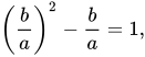
or

${\displaystyle {\frac {b}{a}}=\varphi ,}$

where φ is the golden ratio:

${\displaystyle \varphi ={\frac {1+{\sqrt {5}}}{2}}=1.618033988\ldots }$

The appearance of the golden ratio in the proportional spacing of the evaluation points is how this search algorithm gets its name.

Any number of termination conditions may be applied, depending upon the application. The interval ΔX = X₄ − X₁ is a measure of the absolute error in the estimation of the minimum X and may be used to terminate the algorithm. The value of ΔX is reduced by a factor of r = φ − 1 for each iteration, so the number of iterations to reach an absolute error of ΔX is about ln(ΔX/ΔX₀) / ln(r), where ΔX₀ is the initial value of ΔX.

Because smooth functions are flat (their first derivative is close to zero) near a minimum, attention must be paid not to expect too great an accuracy in locating the minimum. The termination condition provided in the book Numerical Recipes in C is based on testing the gaps among ${\displaystyle x_{1}}$, ${\displaystyle x_{2}}$, ${\displaystyle x_{3}}$ and ${\displaystyle x_{4}}$, terminating when within the relative accuracy bounds

${\displaystyle |x_{3}-x_{1}|<\tau {\big (}|x_{2}|+|x_{4}|{\big )},}$

where ${\displaystyle \tau }$ is a tolerance parameter of the algorithm, and ${\displaystyle |x|}$ is the absolute value of ${\displaystyle x}$. The check is based on the bracket size relative to its central value, because that relative error in ${\displaystyle x}$ is approximately proportional to the squared absolute error in ${\displaystyle f(x)}$ in typical cases. For that same reason, the Numerical Recipes text recommends that ${\displaystyle \tau ={\sqrt {\varepsilon }}}$, where ${\displaystyle \varepsilon }$ is the required absolute precision of ${\displaystyle f(x)}$.

Note! The examples here describe an algorithm that is for finding the minimum of a function. For maximum, the comparison operators need to be reversed.

1. Specify the function to be minimized, ⁠${\displaystyle f(x)}$⁠, the interval to be searched as {X₁,X₄}, and their functional values F₁ and F₄.
2. Calculate an interior point and its functional value F₂. The two interval lengths are in the ratio c : r or r : c where r = φ − 1; and c = 1 − r, with φ being the golden ratio.
3. Using the triplet, determine if convergence criteria are fulfilled. If they are, estimate the X at the minimum from that triplet and return.
4. From the triplet, calculate the other interior point and its functional value. The three intervals will be in the ratio ⁠${\displaystyle c:cr:c}$⁠.
5. The three points for the next iteration will be the one where F is a minimum, and the two points closest to it in X.
6. Go to step 3.

"""
Python program for golden section search.  This implementation
does not reuse function evaluations and assumes the minimum is c
or d (not on the edges at a or b)
"""

import math

invphi = (math.sqrt(5) - 1) / 2  # 1 / phi


def gss(f, a, b, tolerance=1e-5):
    """
    Golden-section search
    to find the minimum of f on [a,b]

    * f: a strictly unimodal function on [a,b]

    Example:
    >>> def f(x): return (x - 2) ** 2
    >>> x = gss(f, 1, 5)
    >>> print(f"{x:.5f}")
    2.00000

    """
    while b - a > tolerance:
        c = b - (b - a) * invphi
        d = a + (b - a) * invphi
        if f(c) < f(d):
            b = d
        else:  # f(c) > f(d) to find the maximum
            a = c

    return (b + a) / 2

// a and c define range to search
// func(x) returns value of function at x to be minimized
function goldenSection(a, c, func) {
  function split(x1, x2) { return x1 + 0.6180339887498949*(x2-x1); }
  var b = split(a, c);
  var bv = func(b);
  while (a != c) {
    var x = split(a, b);
    var xv = func(x);
    if (xv < bv) {
      bv = xv;
      c = b;
      b = x;
    }
    else {
      a = c;
      c = x;
    }
  }
  return b;
}
function test(x) { return -Math.sin(x); }
console.log(goldenSection(0, 3, test)); // prints PI/2

"""
Python program for golden section search.  This implementation
does not reuse function evaluations and assumes the minimum is c
or d (not on the edges at a or b)
"""

import math

invphi = (math.sqrt(5) - 1) / 2  # 1 / phi
invphi2 = (3 - math.sqrt(5)) / 2  # 1 / phi^2


def gss(f, a, b, tolerance=1e-5):
    """
    Golden-section search.

    Given a function f with a single local minimum in
    the interval [a,b], gss returns a subset interval
    [c,d] that contains the minimum with d-c <= tolerance.

    Example:
    >>> def f(x): return (x - 2) ** 2
    >>> print(*gss(f, a=1, b=5, tolerance=1e-5))
    1.9999959837979107 2.0000050911830893
    """
    a, b = min(a, b), max(a, b)
    h = b - a
    if h <= tolerance:
        return (a, b)

    # Required steps to achieve tolerance
    n = int(math.ceil(math.log(tolerance / h) / math.log(invphi)))

    c, d = a + invphi2 * h, a + invphi * h
    yc, yd = f(c), f(d)

    for _ in range(n - 1):
        h *= invphi
        if yc < yd:
            b, d = d, c
            yd = yc
            c = a + invphi2 * h
            yc = f(c)
        else:  # yc > yd to find the maximum
            a, c = c, d
            yc = yd
            d = a + invphi * h
            yd = f(d)

    return (a, d) if yc < yd else (c, b)

public class GoldenSectionSearch {
    public static final double invphi = (Math.sqrt(5.0) - 1) / 2.0;
    public static final double invphi2 = (3 - Math.sqrt(5.0)) / 2.0;

    public interface Function {
        double of(double x);
    }

    // Returns subinterval of [a,b] containing minimum of f

    public static double[] gss(Function f, double a, double b, double tol) {
        return gss(f, a, b, tol, b - a, true, 0, 0, true, 0, 0);
    }
    private static double[] gss(Function f, double a, double b, double tol,
                                double h, boolean noC, double c, double fc,
                                boolean noD, double d, double fd) {
        if (Math.abs(h) <= tol) {
            return new double[] { a, b };
        }
        if (noC) {
            c = a + invphi2 * h;
            fc = f.of(c);
        }
        if (noD) {
            d = a + invphi * h;
            fd = f.of(d);
        }
        if (fc < fd) {  // fc > fd to find the maximum
            return gss(f, a, d, tol, h * invphi, true, 0, 0, false, c, fc);
        } else {
            return gss(f, c, b, tol, h * invphi, false, d, fd, true, 0, 0);
        }
    }

    public static void main(String[] args) {
        Function f = (x)->Math.pow(x-2, 2);
        double a = 1;
        double b = 5;
        double tol = 1e-5;
        double [] ans = gss(f, a, b, tol);
        System.out.println("[" + ans[0] + "," + ans[1] + "]");
        // [1.9999959837979107,2.0000050911830893]
    }
}

import math


invphi = (math.sqrt(5) - 1) / 2  # 1 / phi
invphi2 = (3 - math.sqrt(5)) / 2  # 1 / phi^2


def gssrec(f, a, b, tol=1e-5, h=None, c=None, d=None, fc=None, fd=None):
    """Golden-section search, recursive.

    Given a function f with a single local minimum in
    the interval [a, b], gss returns a subset interval
    [c, d] that contains the minimum with d-c <= tol.

    Example:
    >>> f = lambda x: (x - 2) ** 2
    >>> a = 1
    >>> b = 5
    >>> tol = 1e-5
    >>> (c, d) = gssrec(f, a, b, tol)
    >>> print (c, d)
    1.9999959837979107 2.0000050911830893
    """

    (a, b) = (min(a, b), max(a, b))
    if h is None:
        h = b - a
    if h <= tol:
        return (a, b)
    if c is None:
        c = a + invphi2 * h
    if d is None:
        d = a + invphi * h
    if fc is None:
        fc = f(c)
    if fd is None:
        fd = f(d)
    if fc < fd:  # fc > fd to find the maximum
        return gssrec(f, a, d, tol, h * invphi, c=None, fc=None, d=c, fd=fc)
    else:
        return gssrec(f, c, b, tol, h * invphi, c=d, fc=fd, d=None, fd=None)

A very similar algorithm can also be used to find the extremum (minimum or maximum) of a sequence of values that has a single local minimum or local maximum. In order to approximate the probe positions of golden section search while probing only integer sequence indices, the variant of the algorithm for this case typically maintains a bracketing of the solution in which the length of the bracketed interval is a Fibonacci number. For this reason, the sequence variant of golden section search is often called Fibonacci search.

Fibonacci search was first devised by Kiefer (1953) as a minimax search for the maximum (minimum) of a unimodal function in an interval.

The Bisection method is a similar algorithm for finding a zero of a function. Note that, for bracketing a zero, only two points are needed, rather than three. The interval ratio decreases by 2 in each step, rather than by the golden ratio.

• Ternary search
• Brent's method
• Binary search