Hubbry Logo
Two-dimensional nuclear magnetic resonance spectroscopyTwo-dimensional nuclear magnetic resonance spectroscopyMain
Open search
Two-dimensional nuclear magnetic resonance spectroscopy
Community hub
Two-dimensional nuclear magnetic resonance spectroscopy
logo
8 pages, 0 posts
0 subscribers
Be the first to start a discussion here.
Two-dimensional nuclear magnetic resonance spectroscopy
from Wikipedia
Nuclear Magnetic Resonance (NMR) Spectrometer

Two-Dimensional Nuclear Magnetic Resonance (2D NMR) is an advanced spectroscopic technique that builds upon the capabilities of one-dimensional (1D) NMR by incorporating an additional frequency dimension. This extension allows for a more comprehensive analysis of molecular structures.[1] In 2D NMR, signals are distributed across two frequency axes, providing improved resolution and separation of overlapping peaks, particularly beneficial for studying complex molecules. This technique identifies correlations between different nuclei within a molecule, facilitating the determination of connectivity, spatial proximity, and dynamic interactions.

2D NMR encompasses a variety of experiments,[1] including COSY (Correlation Spectroscopy), TOCSY (Total Correlation Spectroscopy), NOESY (Nuclear Overhauser Effect Spectroscopy), and HSQC (Heteronuclear Single Quantum Coherence). These techniques are indispensable in fields such as structural biology, where they are pivotal in determining protein and nucleic acid structures; organic chemistry, where they aid in elucidating complex organic molecules; and materials science, where they offer insights into molecular interactions in polymers and metal-organic frameworks. By resolving signals that would typically overlap in the 1D NMR spectra of complex molecules, 2D NMR enhances the clarity of structural information.[1] 2D NMR can provide detailed information about the chemical structure and the three-dimensional arrangement of molecules.

The first two-dimensional experiment, COSY, was proposed by Jean Jeener, a professor at the Université Libre de Bruxelles, in 1971. This experiment was later implemented by Walter P. Aue, Enrico Bartholdi and Richard R. Ernst, who published their work in 1976.[2][3][4]

Fundamental concepts

[edit]

Each experiment consists of a sequence of radio frequency (RF) pulses with delay periods in between them. The timing, frequencies, and intensities of these pulses distinguish different NMR experiments from one another.[5] Almost all two-dimensional experiments have four stages: the preparation period, where a magnetization coherence is created through a set of RF pulses; the evolution period, a determined length of time during which no pulses are delivered and the nuclear spins are allowed to freely precess (rotate); the mixing period, where the coherence is manipulated by another series of pulses into a state which will give an observable signal; and the detection period, in which the free induction decay signal from the sample is observed as a function of time, in a manner identical to one-dimensional FT-NMR.[6]

The two dimensions of a two-dimensional NMR experiment are two frequency axes representing a chemical shift. Each frequency axis is associated with one of the two time variables, which are the length of the evolution period (the evolution time) and the time elapsed during the detection period (the detection time). They are each converted from a time series to a frequency series through a two-dimensional Fourier transform. A single two-dimensional experiment is generated as a series of one-dimensional experiments, with a different specific evolution time in successive experiments, with the entire duration of the detection period recorded in each experiment.[6]

The end result is a plot showing an intensity value for each pair of frequency variables. The intensities of the peaks in the spectrum can be represented using a third dimension. More commonly, intensity is indicated using contour lines or different colors.

Homonuclear through-bond correlation methods

[edit]

In these methods, magnetization transfer occurs between nuclei of the same type, through J-coupling of nuclei connected by up to a few bonds.

Correlation spectroscopy (COSY)

[edit]
In standard COSY, the preparation (p1) and mixing (p2) periods each consist of a single 90° pulse separated by the evolution time t1, and the resonance signal from the sample is read during the detection period over a range of times t2.

The first and most popular two-dimension NMR experiment is the homonuclear correlation spectroscopy (COSY) sequence, which is used to identify spins which are coupled to each other. It consists of a single RF pulse (p1) followed by the specific evolution time (t1) followed by a second pulse (p2) followed by a measurement period (t2).[7]

The Correlation Spectroscopy experiment operates by correlating nuclei coupled to each other through scalar coupling, also known as J-coupling.[8] This coupling is the interaction between nuclear spins connected by bonds, typically observed between nuclei that are 2-3 bonds apart (e.g., vicinal protons). By detecting these interactions, COSY provides vital information about the connectivity between atoms within a molecule, making it a crucial tool for structural elucidation in organic chemistry.

The COSY experiment generates a two-dimensional spectrum with chemical shifts along the x-axis (horizontal) and y-axis (vertical) and involves several key steps.[1] First, the sample is excited using a series of radiofrequency (RF) pulses, bringing the nuclear spins into a higher energy state. After the first RF pulse, the system evolves freely for a period called t1, during which the spins precess at frequencies corresponding to their chemical shifts. The correlation between nuclei is achieved by incrementally varying the evolution time (t1) to capture indirect interactions. This series of experiments, each with a different value of t1, allows for the detection of chemical shifts from nuclei that may not be observed directly in a one-dimensional spectrum. As t1 is incremented, cross-peaks are produced in the resulting 2D spectrum, representing interactions like coupling or spatial proximity between nuclei. This approach helps map out atomic connections, providing deeper insight into molecular structure and aiding in the interpretation of complex systems.

Cross peaks result from a phenomenon called magnetization transfer, and their presence indicates that two nuclei are coupled which have the two different chemical shifts that make up the cross peak's coordinates. Each coupling gives two symmetrical cross peaks above and below the diagonal. That is, a cross-peak occurs when there is a correlation between the signals of the spectrum along each of the two axes at these values. An easy visual way to determine which couplings a cross peak represents is to find the diagonal peak which is directly above or below the cross peak, and the other diagonal peak which is directly to the left or right of the cross peak. The nuclei represented by those two diagonal peaks are coupled.[7]

Next, a second RF pulse is applied to allow magnetization to transfer between coupled nuclei. The resulting signal is recorded continuously during a detection period ( t2) after the second RF pulse. The data are then processed through Fourier transformation along both the t1 and t2 axes, creating a 2D spectrum with peaks plotted along the diagonal and off-diagonal.

When interpreting the COSY spectrum, diagonal peaks correspond to the 1D chemical shifts of individual nuclei, similar to the standard peaks in a 1D NMR spectrum. The key feature of a COSY spectrum is the presence of cross-peaks as shown in Figure 1, indicating coupling between pairs of nuclei. These cross-peaks provide crucial information about the connectivity within a molecule, showing that the two nuclei are connected by a small number of bonds, usually two or three bonds.

COSY is especially useful when dealing with complex molecules such as natural products, peptides, and proteins, where understanding the connectivity of different nuclei through bonds is crucial. While 1D NMR is more straightforward and ideal for identifying basic structural features, COSY enhances the capabilities of NMR by providing deeper insights into molecular connectivity.

The two-dimensional spectrum that results from the COSY experiment shows the frequencies for a single isotope, most commonly hydrogen (1H) along both axes. (Techniques have also been devised for generating heteronuclear correlation spectra, in which the two axes correspond to different isotopes, such as 13C and 1H.) Diagonal peaks correspond to the peaks in a 1D-NMR experiment, while the cross peaks indicate couplings between pairs of nuclei (much as multiplet splitting indicates couplings in 1D-NMR).[7]

1H COSY spectrum of progesterone. The spectrum that appears along both the horizontal and vertical axes is a regular one dimensional 1H NMR spectrum. The bulk of the peaks appear along the diagonal, while cross-peaks appear symmetrically above and below the diagonal.

COSY-90 is the most common COSY experiment. In COSY-90, the p1 pulse tilts the nuclear spin by 90°. Another member of the COSY family is COSY-45. In COSY-45 a 45° pulse is used instead of a 90° pulse for the second pulse, p2. The advantage of a COSY-45 is that the diagonal-peaks are less pronounced, making it simpler to match cross-peaks near the diagonal in a large molecule. Additionally, the relative signs of the coupling constants (see J-coupling#Magnitude of J-coupling) can be elucidated from a COSY-45 spectrum. This is not possible using COSY-90.[9] Overall, the COSY-45 offers a cleaner spectrum while the COSY-90 is more sensitive.

Another related COSY technique is double quantum filtered (DQF) COSY. DQF COSY uses a coherence selection method such as phase cycling or pulsed field gradients, which cause only signals from double-quantum coherences to give an observable signal. This has the effect of decreasing the intensity of the diagonal peaks and changing their lineshape from a broad "dispersion" lineshape to a sharper "absorption" lineshape. It also eliminates diagonal peaks from uncoupled nuclei. These all have the advantage that they give a cleaner spectrum in which the diagonal peaks are prevented from obscuring the cross peaks, which are weaker in a regular COSY spectrum.[10]

Exclusive correlation spectroscopy (ECOSY)

[edit]

Total correlation spectroscopy (TOCSY)

[edit]
Typical TOCSY values for amino acids

The TOCSY experiment is similar to the COSY experiment, in that cross peaks of coupled protons are observed. However, cross peaks are observed not only for nuclei which are directly coupled, but also between nuclei which are connected by a chain of couplings. This makes it useful for identifying the larger interconnected networks of spin couplings. This ability is achieved by inserting a repetitive series of pulses which cause isotropic mixing during the mixing period. Longer isotropic mixing times cause the polarization to spread out through an increasing number of bonds.[11]

In the case of oligosaccharides, each sugar residue is an isolated spin system, so it is possible to differentiate all the protons of a specific sugar residue. A 1D version of TOCSY is also available, and by irradiating a single proton the rest of the spin system can be revealed. Recent advances in this technique include the 1D-CSSF (chemical shift selective filter) TOCSY experiment, which produces higher quality spectra and allows coupling constants to be reliably extracted and used to help determine stereochemistry.

TOCSY is sometimes called "homonuclear Hartmann–Hahn spectroscopy" (HOHAHA).[12]

Incredible natural-abundance double-quantum transfer experiment (INADEQUATE)

[edit]

INADEQUATE[13] is a method often used to find 13C couplings between adjacent carbon atoms. Because the natural abundance of 13C is only about 1%, only about 0.01% of molecules being studied will have the two nearby 13C atoms needed for a signal in this experiment. However, correlation selection methods are used (similarly to DQF COSY) to prevent signals from single 13C atoms, so that the double 13C signals can be easily resolved. Each coupled pair of nuclei gives a pair of peaks on the INADEQUATE spectrum which both have the same vertical coordinate, which is the sum of the chemical shifts of the nuclei; the horizontal coordinate of each peak is the chemical shift for each of the nuclei separately.[14]

Heteronuclear through-bond correlation methods

[edit]

Heteronuclear correlation spectroscopy gives signal based upon coupling between nuclei of two different types. Often the two nuclei are protons and another nucleus (called a "heteronucleus"). For historical reasons, experiments which record the proton rather than the heteronucleus spectrum during the detection period are called "inverse" experiments. This is because the low natural abundance of most heteronuclei would result in the proton spectrum being overwhelmed with signals from molecules with no active heteronuclei, making it useless for observing the desired, coupled signals. With the advent of techniques for suppressing these undesired signals, inverse correlation experiments such as HSQC, HMQC, and HMBC are actually much more common today. "Normal" heteronuclear correlation spectroscopy, in which the heteronucleus spectrum is recorded, is known as HETCOR.[15]

Heteronuclear single-quantum correlation spectroscopy (HSQC)

[edit]
1H–15N HSQC spectrum of a fragment of the protein NleG3-2. Each peak in the spectrum represents a bonded N–H pair, with its two coordinates corresponding to the chemical shifts of each of the H and N atoms. Some of the peaks are labeled with the amino acid residue that gives that signal.[16]

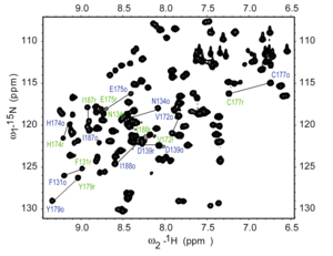
Heteronuclear Single Quantum Coherence (HSQC) is a 2D NMR technique utilized for the detection of interactions between different types of nuclei which are separated by one bond, particularly a proton (1H) and a heteronucleus such as carbon (13C) or nitrogen (15N).[17] This method gives one peak per pair of coupled nuclei, whose two coordinates are the chemical shifts of the two coupled atoms.[18]

This method plays a role in structural elucidation, particularly in analyzing organic compounds, natural products, and biomolecules such as proteins and nucleic acids. HSQC is designed to detect one-bond correlations between protons and heteronuclear atoms, providing insight into the connectivity of hydrogen and heteronuclear atoms through the transfer of magnetization.

The HSQC experiment involves a series of steps to generate a two-dimensional NMR spectrum. Initially, the sample is excited using radiofrequency (RF) pulses, bringing the nuclear spins into an excited state and preparing them for magnetization transfer. Magnetization is then transferred from the proton to the heteronucleus through a one-bond scalar coupling (J-coupling), ensuring that only directly bonded nuclei participate in the transfer. Subsequently, the system evolves during a period called t1, and the magnetization is transferred back from the heteronuclear to the proton. The final signal is detected, encoding both the proton and the heteronuclear information, and a Fourier transformation is performed to create a 2D spectrum correlating the proton and heteronuclear chemical shifts.

HSQC works by transferring magnetization from the I nucleus (usually the proton) to the S nucleus (usually the heteroatom) using the INEPT pulse sequence; this first step is done because the proton has a greater equilibrium magnetization and thus this step creates a stronger signal. The magnetization then evolves and then is transferred back to the I nucleus for observation. An extra spin echo step can then optionally be used to decouple the signal, simplifying the spectrum by collapsing multiplets to a single peak. The undesired uncoupled signals are removed by running the experiment twice with the phase of one specific pulse reversed; this reverses the signs of the desired but not the undesired peaks, so subtracting the two spectra will give only the desired peaks.[18]

Interpretation of the HSQC spectrum is based on the observation of cross-peaks, which indicates the direct bonding between protons and carbons or nitrogens. Each cross-peak corresponds to a specific 1H-13C or 1H-15N pair, providing direct assignments of 1H-Xconnectivity, where X is the heteronucleus[17] The HSQC technique offers several advantages, including its focus on one-bond correlations, increased sensitivity due to the direct detection of protons, and the simplification of crowded spectra by resolving overlapping signals and aiding in the analysis of complex molecules.

Heteronuclear multiple-quantum correlation spectroscopy (HMQC) gives an identical spectrum as HSQC, but using a different method. The two methods give similar quality results for small to medium-sized molecules, but HSQC is considered to be superior for larger molecules.[18]

Heteronuclear multiple-bond correlation spectroscopy (HMBC)

[edit]

HMBC detects heteronuclear correlations over longer ranges of about 2–4 bonds. The difficulty of detecting multiple-bond correlations is that the HSQC and HMQC sequences contain a specific delay time between pulses which allows detection only of a range around a specific coupling constant. This is not a problem for the single-bond methods since the coupling constants tend to lie in a narrow range, but multiple-bond coupling constants cover a much wider range and cannot all be captured in a single HSQC or HMQC experiment.[19]

In HMBC, this difficulty is overcome by omitting one of these delays from an HMQC sequence. This increases the range of coupling constants that can be detected, and also reduces signal loss from relaxation. The cost is that this eliminates the possibility of decoupling the spectrum, and introduces phase distortions into the signal. There is a modification of the HMBC method which suppresses one-bond signals, leaving only the multiple-bond signals.[19]

Through-space correlation methods

[edit]

These methods establish correlations between nuclei which are physically close to each other regardless of whether there is a bond between them. They use the nuclear Overhauser effect (NOE) by which nearby atoms (within about 5 Å) undergo cross relaxation by a mechanism related to spin–lattice relaxation.

Nuclear Overhauser effect spectroscopy (NOESY)

[edit]

In NOESY, the nuclear Overhauser cross relaxation between nuclear spins during the mixing period is used to establish the correlations. The spectrum obtained is similar to COSY, with diagonal peaks and cross peaks, however the cross peaks connect resonances from nuclei that are spatially close rather than those that are through-bond coupled to each other. NOESY spectra also contain extra axial peaks which do not provide extra information and can be eliminated through a different experiment by reversing the phase of the first pulse.[20]

One application of NOESY is in the study of large biomolecules, such as in protein NMR, in which relationships can often be assigned using sequential walking.

The NOESY experiment can also be performed in a one-dimensional fashion by pre-selecting individual resonances. The spectra are read with the pre-selected nuclei giving a large, negative signal while neighboring nuclei are identified by weaker, positive signals. This only reveals which peaks have measurable NOEs to the resonance of interest but takes much less time than the full 2D experiment. In addition, if a pre-selected nucleus changes environment within the time scale of the experiment, multiple negative signals may be observed. This offers exchange information similar to the EXSY (exchange spectroscopy) NMR method.

NOESY experiments are important tool to identify stereochemistry of a molecule in solvent whereas single crystal XRD used to identify stereochemistry of a molecule in solid form.

Heteronuclear Overhauser effect spectroscopy (HOESY)

[edit]

In HOESY, much like NOESY is used for the cross relaxation between nuclear spins. However, HOESY can offer information about other NMR active nuclei in a spatially relevant manner. Examples include any nuclei X{Y} or X→Y such as 1H→13C, 19F→13C, 31P→13C, or 77Se→13C. The experiments typically observe NOEs from protons on X, X{1H}, but do not have to include protons.[21]

Rotating-frame nuclear Overhauser effect spectroscopy (ROESY)

[edit]

ROESY is similar to NOESY, except that the initial state is different. Instead of observing cross relaxation from an initial state of z-magnetization, the equilibrium magnetization is rotated onto the x axis and then spin-locked by an external magnetic field so that it cannot precess. This method is useful for certain molecules whose rotational correlation time falls in a range where the nuclear Overhauser effect is too weak to be detectable, usually molecules with a molecular weight around 1000 daltons, because ROESY has a different dependence between the correlation time and the cross-relaxation rate constant. In NOESY the cross-relaxation rate constant goes from positive to negative as the correlation time increases, giving a range where it is near zero, whereas in ROESY the cross-relaxation rate constant is always positive.[22][23]

ROESY is sometimes called "cross relaxation appropriate for minimolecules emulated by locked spins" (CAMELSPIN).[23]

Resolved-spectrum methods

[edit]

Unlike correlated spectra, resolved spectra spread the peaks in a 1D-NMR experiment into two dimensions without adding any extra peaks. These methods are usually called J-resolved spectroscopy, but are sometimes also known as chemical shift resolved spectroscopy or δ-resolved spectroscopy. They are useful for analysing molecules for which the 1D-NMR spectra contain overlapping multiplets as the J-resolved spectrum vertically displaces the multiplet from each nucleus by a different amount. Each peak in the 2D spectrum will have the same horizontal coordinate that it has in a non-decoupled 1D spectrum, but its vertical coordinate will be the chemical shift of the single peak that the nucleus has in a decoupled 1D spectrum.[24]

For the heteronuclear version, the simplest pulse sequence used is called a Müller–Kumar–Ernst (MKE) experiment, which has a single 90° pulse for the heteronucleus for the preparation period, no mixing period, and applies a decoupling signal to the proton during the detection period. There are several variants on this pulse sequence which are more sensitive and more accurate, which fall under the categories of gated decoupler methods and spin-flip methods. Homonuclear J-resolved spectroscopy uses the spin echo pulse sequence.[24]

Higher-dimensional methods

[edit]

3D and 4D experiments can also be done, sometimes by running the pulse sequences from two or three 2D experiments in series. Many of the commonly used 3D experiments, however, are triple resonance experiments; examples include the HNCA and HNCOCA experiments, which are often used in protein NMR.

See also

[edit]

References

[edit]
Revisions and contributorsEdit on WikipediaRead on Wikipedia
from Grokipedia
Two-dimensional (2D NMR) is an advanced analytical technique that extends traditional one-dimensional NMR by spreading spectral information across two frequency dimensions, enabling the correlation of nuclear spins through interactions such as and nuclear Overhauser effects (NOE), thereby resolving signal overlaps and revealing molecular connectivity and spatial arrangements in complex samples. This method significantly enhances and provides detailed structural insights, particularly for biomolecules and organic compounds, by generating contour plots where peaks indicate relationships between nuclei. The development of 2D NMR traces back to a 1971 lecture by James Jeener, who proposed the concept of correlating spin evolutions over two time periods, though it remained unpublished until Richard R. Ernst and colleagues formalized and implemented it in 1976 using Fourier transform techniques. Ernst's pioneering work on multidimensional NMR earned him the Nobel Prize in Chemistry in 1991, while Kurt Wüthrich's applications to protein structure determination using 2D and higher-dimensional methods led to his Nobel in 2002. These advancements built on the earlier shift to Fourier transform NMR in the 1960s, transforming NMR from a time-consuming tool into a multidimensional powerhouse for spectroscopy. At its core, 2D NMR operates through a pulse sequence divided into four periods: preparation, evolution (t1), mixing, and detection (t2), where the evolution time encodes one frequency dimension and detection captures the other, followed by double Fourier transformation to produce the 2D spectrum. Common variants include homonuclear experiments like COSY (correlation spectroscopy), which detects to map through-bond connectivities, and NOESY ( Spectroscopy), which reveals through-space proximities via NOE; heteronuclear methods such as HSQC (heteronuclear single quantum coherence) correlate protons with 13C or 15N nuclei, crucial for isotopic-labeled samples. These techniques exploit coherence transfer and multiple quantum coherences to amplify weak signals and simplify crowded spectra. In practice, 2D NMR has revolutionized fields like , , and pharmaceuticals by facilitating the assignment of resonances in proteins up to ~50 kDa, determining three-dimensional structures, and studying dynamics and interactions. Applications extend to for ligand binding analysis and material sciences for , with ongoing innovations like ultrafast 2D methods reducing acquisition times from hours to seconds. Despite challenges such as sensitivity limitations for large molecules, isotope labeling and higher-field magnets continue to expand its utility.

Fundamental Principles

Transition from 1D to 2D NMR

One-dimensional (1D) (NMR) spectroscopy excels at providing and integration data for simple molecules but faces significant challenges with signal overlap in complex systems, such as biomolecules or synthetic polymers, where resonances from multiple nuclei crowd into a limited spectral window. This overlap obscures individual peak assignments and prevents reliable determination of scalar (J) couplings, which are crucial for inferring through-bond connectivity. Additionally, 1D NMR offers no direct insight into spatial proximities between non-equivalent nuclei, limiting its utility for full structural elucidation in crowded spectra. To overcome these constraints, two-dimensional (2D) NMR techniques emerged in the as a means to deconvolute spectral complexity by distributing information across an additional dimension, thereby resolving ambiguities inherent in 1D data. The motivation stemmed from the need to handle increasingly complex samples in organic and biochemical research, where traditional 1D methods failed to separate overlapping signals in high-field spectra. Pivotal early work by , Bartholdi, and in demonstrated the practical implementation of 2D (FT) NMR, applying it to simple spin systems to showcase enhanced resolution for multiple quantum transitions and mapping. At its core, 2D NMR achieves resolution by correlating frequencies along two axes: the direct dimension (F2), acquired through standard signal detection as in 1D NMR, and the indirect dimension (F1), encoded via time increments during a preparation period to capture evolution of coherences. This bivariate representation spreads and coupling information, allowing cross-peaks to reveal relationships between nuclei that appear superimposed in 1D. For instance, J-coupled multiplets from adjacent protons that overlap in a 1D proton —such as methylene groups in a —can be separated in 2D space, with their distinct shifts appearing along the F1 axis while couplings manifest as fine structure along F2, facilitating unambiguous assignment.

Core Elements of the 2D Experiment

The two-dimensional (2D NMR) experiment follows a universal pulse sequence structure consisting of four distinct periods: preparation, evolution, mixing, and detection. These periods enable the encoding and correlation of nuclear spin interactions across two dimensions, addressing limitations of one-dimensional NMR by resolving overlapping signals. In the preparation period, radiofrequency pulses initially excite the nuclear spins from equilibrium, creating transverse that serves as the starting point for subsequent evolution. The evolution period (t₁) follows, during which the precesses freely under and interactions, encoding information in the indirect without direct signal acquisition. The mixing period then transfers coherence between spins via pulses or delays, allowing correlations to form between the evolutions in t₁ and the subsequent detection. Finally, the detection period (t₂) records the (FID) in the direct , capturing the modulated signal as a function of time. Coherence transfer pathways define the evolution of spin orders throughout the sequence, ensuring only desired interactions contribute to the signal while suppressing artifacts. These pathways are selected using phase cycling, where the phases of pulses and the receiver are systematically varied over multiple scans to retain coherences with specific order changes (e.g., from single-quantum to zero-quantum), or pulsed field gradients, which dephase unwanted pathways based on spatial encoding. Encoding in the indirect relies on incrementing the time t₁ in small, regular steps (typically 50–500 increments) across successive scans, building a matrix of interferograms that map . Quadrature detection in this , achieved by alternating the phase of the receiver or using methods like States-TPPI, simultaneously records real and imaginary components to distinguish positive and negative , preventing artifacts such as quadrature images. The resulting time-domain signal can be expressed as S(t1,t2)=M(t1)exp(iΩ2t2)S(t_1, t_2) = M(t_1) \exp(i \Omega_2 t_2), where M(t1)M(t_1) reflects the evolution and coherence transfer during t₁ and mixing, modulating the detection signal during t₂. Relaxation processes, particularly transverse relaxation (T₂), occur throughout the periods and attenuate signal intensity, with decay exponential in t₁, mixing, and t₂, leading to broader peaks and reduced sensitivity for longer experiments. Longitudinal relaxation (T₁) during preparation influences recovery between scans, while differential T₂ effects across spins can distort cross-peak intensities, necessitating optimization of period durations to balance resolution and signal-to-noise./01:_Basic_NMR_Theory/1.10:_How_do_T_and_T_relaxation_affect_NMR_spectra)

Data Acquisition and Processing

In two-dimensional (2D NMR) spectroscopy, involves systematically varying the evolution time t1t_1 in the indirect dimension while acquiring free induction decays (FIDs) in the direct dimension t2t_2. Typically, the number of t1t_1 increments ranges from 256 to 1024 points to achieve adequate resolution in the F1 dimension, though smaller sets like 128 or 512 may suffice for initial surveys. The spectral width is set in both dimensions to encompass the expected resonances, often 10-20 ppm for homonuclear 1H^1\mathrm{H} experiments in F2 and F1, or wider (e.g., 160-220 ppm) in F1 for heteronuclear correlations to cover 13C^{13}\mathrm{C} or other nuclei. A relaxation delay of 1-3 seconds is commonly employed between scans to allow recovery, scaled to approximately 1.25 times the longest T1T_1 relaxation time for efficiency. The acquired time-domain signal matrix s(t1,t2)s(t_1, t_2) is transformed into the frequency-domain spectrum S(ω1,ω2)S(\omega_1, \omega_2) via a two-dimensional (2D FT), performed first along t2t_2 to yield a series of 1D spectra, then along t1t_1. The 2D FT is mathematically expressed as S(ω1,ω2)=s(t1,t2)eiω1t1eiω2t2dt1dt2,S(\omega_1, \omega_2) = \iint s(t_1, t_2) \, e^{-i \omega_1 t_1} \, e^{-i \omega_2 t_2} \, dt_1 \, dt_2, resulting in an F1-F2 frequency matrix that encodes correlations between nuclear spins. This process, foundational to 2D NMR, separates overlapping resonances into distinct peaks across two frequency axes. Processing begins with zero-filling, where the data matrix is padded with zeros to double or quadruple its size in each dimension, enhancing digital resolution without introducing new information. Window functions are then applied to the FIDs to optimize the between resolution and sensitivity; for example, a shifted sine-bell function (e.g., QSINE with shift 0-2) is often used for COSY-like data to suppress truncation artifacts while preserving peak sharpness. Phasing follows in both dimensions, typically starting with zero-order (PHC0) and first-order (PHC1) corrections to achieve pure absorption lineshapes, performed manually or automatically after the initial FT. Common artifacts include t1t_1 noise, manifesting as striped patterns parallel to the F1 axis due to imperfect receiver gain or phase cycling, and diagonal artifacts arising from incomplete suppression of axial peaks or field inhomogeneities. These are mitigated by symmetrization along the diagonal for magnitude-mode spectra or by adjusting acquisition parameters like dummy scans (16-32). Baseline correction employs polynomial fitting (order 2-5) to subtract low-frequency distortions in both dimensions, ensuring flat baselines for accurate integration. Spectra are displayed in various modes to suit the experiment: magnitude mode, where peaks appear as absolute values S(ω1,ω2)|S(\omega_1, \omega_2)|, is robust for correlation maps with phase inconsistencies but loses information; phase-sensitive mode uses real or imaginary parts after proper phasing for dispersive or absorptive lineshapes, enabling detection of cross-peak signs in NOESY or TOCSY. Real-part displays are preferred for high-resolution phase-sensitive spectra, while imaginary parts may highlight quadrature artifacts if present.

Through-Bond Homonuclear Correlation Methods

Correlation Spectroscopy (COSY)

Correlation (COSY) is a pioneering two-dimensional NMR method that reveals homonuclear correlations between protons connected through scalar J-couplings, enabling the mapping of spin networks in molecules. Developed by Bax and Freeman in 1981, it builds on Jeener's conceptual framework by providing a practical implementation for resolving spectral overlap in one-dimensional NMR.90045-7) The standard COSY pulse sequence begins with a 90° radiofrequency to create transverse , followed by the evolution period t1t_1 during which spins precess under and influences, an incrementable delay essential for encoding the first frequency dimension. A second 90° then serves as the mixing element, transferring coherence between coupled spins, after which the signal is acquired during the detection period t2t_2. This sequence operates within the general phases of preparation, evolution, mixing, and detection typical of 2D NMR experiments.90045-7) The correlation arises from the evolution of antiphase during t1t_1, where converts in-phase signals to antiphase forms for interacting spins; the mixing pulse refocuses and interchanges this antiphase component between coupled protons ii and jj, yielding cross-peaks symmetrically positioned at coordinates (δi,δj)(\delta_i, \delta_j) and (δj,δi)(\delta_j, \delta_i) in the 2D spectrum. Only protons with significant through-bond (typically ¹H-¹H values of 1–20 Hz for vicinal or pairs) produce observable cross-peaks, with the diagonal ridge at (δi,δi)(\delta_i, \delta_i) representing auto-correlations.90045-7) A key variant, double-quantum filtered COSY (DQF-COSY), incorporates an additional 90°-90° filter pair before acquisition to select double-quantum coherence, effectively suppressing signals from singlets and reducing diagonal peak intensity, which enhances visibility of weak cross-peaks in complex spectra. This modification, introduced by Marion and Wüthrich in 1983, is particularly useful for proteins and crowded proton regions.91225-1) COSY spectra exhibit characteristic peak patterns: the diagonal peaks mirror the 1D spectrum, while cross-peaks display from active couplings (between the two correlated ) and passive couplings (to remote ), often manifesting as antiphase multiplets with four-line patterns for isolated AX systems. Axial peaks, artifacts parallel to the axes, arise from incomplete phase cycling and can be minimized through improved acquisition protocols.90045-7) The intensity of a COSY cross-peak is proportional to sin(πJt1)sin(πJtmix)\sin(\pi J t_1) \sin(\pi J t_{\text{mix}}), where JJ is the and tmixt_{\text{mix}} represents a short effective mixing duration following the second ; in basic implementations, tmixt_{\text{mix}} is near zero, making intensity primarily dependent on the t1t_1 evolution for optimal signal at t11/(2J)t_1 \approx 1/(2J). In applications, COSY excels at establishing simple proton connectivities in small molecules (up to ~500 Da), such as identifying vicinal couplings in carbohydrates or alkaloids, thereby aiding rapid structure determination without isotopic labeling.90045-7)

Exclusive Correlation Spectroscopy (ECOSY)

Exclusive Correlation Spectroscopy (ECOSY) serves as an extension of correlation spectroscopy (COSY), utilizing passive heteronuclear couplings to resolve the absolute signs of homonuclear J-couplings in three-spin systems. Introduced in 1985 by Christian Griesinger, Ole W. Sørensen, and , this technique was developed to facilitate stereochemical analysis in organic molecules by exploiting the displacement of cross-peak multiplets. The core principle of ECOSY relies on a passive third spin, such as ^{13}C in an H-H-^{13}C system, which acts as a label to modulate the cross-peak . During the period, the large one-bond ^{1}J(CH) passive causes a displacement of the cross-peak components along the F1 , with the direction of displacement indicating the relative sign between the active homonuclear ^{n}J(HH) and the passive ^{1}J(CH) s. This displacement arises because the passive effectively changes sign due to the refocusing mechanism, allowing the sign of ^{n}J(HH)—typically positive for vicinal couplings—to be determined relative to the known positive ^{1}J(CH).90403-5) The pulse sequence in ECOSY mirrors the standard COSY framework but incorporates a selective 180° on the heteronucleus (e.g., ^{13}C) applied at the midpoint of the t_1 evolution period. This heteronuclear 180° refocuses evolution of the passive spin while inverting the effective sign of the passive during the second half of t_1, resulting in cross-peaks where components are separated by either the sum or difference of ^{1}J(CH) and ^{n}J(HH), depending on their relative signs.90403-5) Analysis of ECOSY cross-peaks involves measuring the vector displacement between multiplet components, where the cross-peak is simplified to antiphase doublets displaced by ^{1}J(CH) ≈ 125–145 Hz in the F1 dimension and split by ^{n}J(HH) in the F2 dimension. This pattern enables stereochemical assignments, such as distinguishing erythro and threo configurations in coupled CH-CH systems, by correlating the observed displacement direction with known J-sign conventions.90403-5) A key limitation of ECOSY is its dependence on observable passive couplings, which at natural ^{13}C abundance (1.1%) yields low sensitivity due to the small population of isotopomers containing ^{13}C. Consequently, the technique often requires ^{13}C-labeled samples to achieve sufficient signal-to-noise ratios for practical applications, particularly in complex molecules.90024-8)

Total Correlation Spectroscopy (TOCSY)

Total Correlation Spectroscopy (TOCSY) is a homonuclear two-dimensional NMR technique that correlates all protons within a coupled spin system by transferring through multiple J-couplings, extending beyond the direct neighbors observed in COSY experiments. This method achieves isotropic mixing of spin states under a strong radio-frequency field, effectively averaging chemical shift differences and allowing efficient propagation of coherence along scalar-coupled chains. Introduced in the mid-1980s, TOCSY builds on the principles of to map entire multiplets, facilitating the identification of isolated spin networks in complex molecules. The core mechanism of TOCSY relies on Hartmann-Hahn mixing during a spin-lock period, where a continuous radio-frequency field locks the in the rotating frame and recouples isotropic J-interactions. In this regime, the effective Hamiltonian simplifies to an isotropic form that promotes uniform transfer of transverse between all coupled spins, regardless of the number of intervening bonds, as long as the constants are comparable. This contrasts with relay mechanisms in COSY variants, which rely on antiphase states and limit transfer to adjacent s; in TOCSY, coherence spreads efficiently through the entire spin system under the spin-lock, though relaxation during the mixing period can attenuate distant correlations. A standard TOCSY pulse sequence begins with a 90° excitation pulse to create transverse , followed by evolution during t₁, then a spin-lock mixing period using sequences like MLEV-16 or DIPSI-2, and finally acquisition in t₂. The MLEV-16 sequence, an improvement over earlier MLEV-17, applies a train of phase-alternating pulses to achieve the Hartmann-Hahn condition over a wide bandwidth, typically 5-10 kHz, minimizing offsets. DIPSI variants offer better performance for weaker fields or broader spectral widths by optimizing pulse phases for more uniform mixing. In TOCSY spectra, cross-peaks appear between all protons belonging to the same multiplet, forming a network that reveals the full extent of the spin system; for example, in an AA'BB' system, every A proton correlates with every B proton, unlike COSY where only adjacent pairs are prominent. The intensity of these cross-peaks diminishes with distance from the source due to T₂ relaxation, but short mixing times emphasize direct couplings while longer ones highlight remote ones. Transfer efficiency in TOCSY is governed by the mixing time τ_m, with the amplitude of magnetization transfer between two spins i and j approximated by sinusoidal functions involving the effective coupling J_eff under isotropic mixing: for a simple two-spin system, it follows I_{ij} \propto \sin^2(\pi J \tau_m / 2) in the weak coupling limit, but approaches uniform distribution (equal transfer to all partners) in the strong coupling regime where the spin-lock field greatly exceeds the J-couplings. Early implementations were termed HOHAHA (homonuclear Hartmann-Hahn spectroscopy), reflecting the mixing , and used MLEV-17 pulses. Variants like z-filtered TOCSY incorporate a z-filter (a pair of 90° pulses with a delay) after mixing to suppress unwanted zero-quantum coherences and axial peaks, improving spectral purity and reducing artifacts from chemical exchange or cross-relaxation. TOCSY finds key applications in assigning spin systems of biomolecules, particularly in carbohydrates where it delineates isolated networks like those in AA'BB' or AMX patterns of sugar residues, aiding structural elucidation of oligosaccharides and glycoconjugates. For instance, in analysis, TOCSY maps the full proton connectivity within each unit, complementing heteronuclear methods for complete assignment.

Incredible Natural-Abundance Double-Quantum Transfer Experiment (INADEQUATE)

The Incredible Natural-Abundance Double-Quantum Transfer Experiment (INADEQUATE) is a homonuclear two-dimensional NMR spectroscopy method specifically tailored to map direct through-bond carbon-carbon connectivities by detecting one-bond scalar couplings (^1J_{CC}) between ^{13}C nuclei at their natural abundance of approximately 1.1%. Introduced as a means to overcome the challenges of low-abundance ^{13}C-^{13}C pairs, it excels in providing unequivocal adjacency information for the carbon skeleton in organic molecules, particularly when proton signals are ambiguous or absent. The core principle of INADEQUATE involves the selective excitation and indirect detection of double-quantum (DQ) coherence arising from rare, naturally occurring pairs of magnetically coupled ^{13}C atoms, which represent only about 0.01% probability for adjacent carbons due to the quadratic dependence on ^{13}C abundance. During the experiment, transverse is converted into antiphase DQ states through precise timing matched to ^1J_{CC}, allowing evolution under differences in the indirect dimension without diagonal peaks that could obscure weak signals. Broadband decoupling of ^1H nuclei is applied to eliminate heteronuclear splittings and enhance resolution.90258-3) The sequence begins with a DQ preparation period: a 90° creates transverse , followed by a delay τ, a 180° refocusing to compensate for evolution, another delay τ, and a second 90° to generate DQ coherence. This is succeeded by the indirect evolution period t_1, during which the DQ signal precesses at the sum of the coupled chemical shifts; a final 90° then reconverts the DQ coherence to single-quantum (SQ) for direct acquisition during t_2 under ^1H decoupling. The delays τ are optimized to approximately 1/(2^1J_{CC}), typically 8-14 ms for common aliphatic ^1J_{CC} values of 30-60 Hz. In the resulting 2D spectrum, cross-peaks for each ^1J_{CC}-coupled pair appear symmetrically at the average chemical shift (ν_i + ν_j)/2 in the F1 (DQ) dimension and at the full chemical shift ν_i or ν_j in the F2 (SQ) dimension, with peak intensities directly proportional to the coupling magnitude ^1J_{CC}, facilitating easy tracing of carbon chains as connected pairs without overlap from unrelated signals. Antiphase multiplet structure along F2 may require processing or refocusing variants for phase-sensitive display.90258-3) Sensitivity remains a primary limitation, as the signal arises solely from the ~0.01% fraction of ^{13}C-^{13}C pairs, yielding intensities roughly 10,000 times weaker than standard ^{13}C spectra and necessitating extended acquisition times—often 1-3 days with hundreds of increments in t_1—and high sample concentrations (e.g., 0.5-1 M for molecules up to 300 Da). Phase cycling or gradient selection helps suppress artifacts, but overall, INADEQUATE demands careful optimization to avoid truncation or low signal-to-noise. The DQ signal intensity generated in the preparation period follows I \propto n_{^{13}C}^2 \sin^2(\pi ^1J_{CC} \tau), where n_{^{13}C} is the natural abundance (~1.1%), underscoring the quadratic sensitivity penalty; maximum transfer occurs at \tau = 1/(2^1J_{CC}), balancing excitation efficiency against relaxation losses.90258-3) Applications of INADEQUATE center on establishing definitive carbon backbone connectivity in unlabeled organic compounds, such as natural products or complex mixtures, where it uniquely confirms direct C-C adjacencies (e.g., in or taxol precursors) without isotopic enrichment, complementing indirect methods in structure elucidation.

Through-Bond Heteronuclear Correlation Methods

Heteronuclear Single-Quantum Correlation Spectroscopy (HSQC)

Heteronuclear single-quantum correlation (HSQC) spectroscopy is a two-dimensional NMR technique that establishes direct one-bond correlations between protons (¹H) and heteronuclei, most commonly ¹³C, by transferring polarization from the high-sensitivity ¹H to the low-sensitivity ¹³C nucleus and detecting the signal on ¹H. Introduced in its foundational form for ¹⁵N detection by Bodenhausen and Ruben in 1980, HSQC has become a cornerstone for ¹H-¹³C correlations due to its superior resolution and sensitivity in mapping chemical environments. The pulse sequence for HSQC begins with an INEPT block to transfer longitudinal ¹H magnetization to antiphase ¹³C magnetization: a 90° pulse on ¹H, followed by a delay τ (typically 1/(4¹J_CH) ≈ 1.8 ms for ¹J_CH ≈ 140 Hz), a simultaneous 180° pulse on both nuclei, another τ delay, and 90° pulses on both nuclei to create transverse ¹³C coherence. During the indirect evolution period t₁, the ¹³C chemical shift is encoded while a 180° pulse on ¹H refocuses heteronuclear J-coupling evolution, effectively decoupling the spectrum in the F₁ dimension. A reverse INEPT then transfers the ¹³C antiphase coherence back to in-phase ¹H magnetization for direct detection under broadband ¹³C decoupling, yielding a high-resolution ¹H-detected spectrum. Cross-peaks in the HSQC spectrum appear at coordinates (δ_¹³C, δ_¹H) corresponding to directly attached proton-carbon pairs, with antiphase multiplets along F₂ collapsed by decoupling; the typical ¹J_CH coupling constant is around 140 Hz, optimizing the transfer efficiency. A phase-sensitive variant of HSQC incorporates elements akin to Distortionless Enhancement by Polarization Transfer (DEPT) during the reverse INEPT, modulating the sign of cross-peaks based on carbon multiplicity: CH and CH₃ groups yield positive-phase peaks, while CH₂ groups appear negative, facilitating distinction without additional experiments. This editing is achieved by adjusting the final ¹³C refocusing delay, preserving overall sensitivity while providing structural insights into hybridization. The sensitivity of HSQC allows for 32- to 64-fold reductions in acquisition time compared to proton-decoupled ¹³C experiments, primarily due to ¹H observation and INEPT enhancement, enabling spectra from quantities of sample in minutes. This gain allows for 32- to 64-fold reductions in acquisition time compared to proton-decoupled ¹³C experiments, making HSQC ideal for low-abundance or dilute samples. In biomolecular applications, HSQC excels at assigning ¹³C resonances by correlating them to resolved ¹H signals, particularly in isotopically labeled proteins where it maps backbone and aliphatic side-chain carbons, aiding secondary and dynamics studies. For instance, in uniformly ¹³C-enriched proteins, HSQC provides a "" spectrum for rapid quality assessment and sequential assignments when combined with triple-resonance experiments.

Heteronuclear Multiple-Bond Correlation Spectroscopy (HMBC)

Heteronuclear Multiple-Bond Correlation Spectroscopy (HMBC) is a two-dimensional NMR technique designed to detect long-range heteronuclear couplings, typically 2J and 3J (and occasionally 4J), between protons and low-abundance nuclei like ¹³C, enabling the mapping of multi-bond connectivities in molecules. Introduced by Bax and Summers in 1986, the method employs a low-pass J-filter to suppress dominant one-bond couplings (¹J), which are usually much larger (120–160 Hz for ¹H–¹³C), while allowing evolution of smaller long-range couplings (2–10 Hz) through delayed magnetization transfer. This selective detection is achieved via multiple-quantum coherence pathways or fixed delays tuned to the expected range of long-range J values, providing indirect structural information beyond direct attachments. The sequence for HMBC resembles that of HSQC but incorporates specific modifications for long-range selectivity, starting with a 90° excitation on the high-γ nucleus (e.g., ¹H), followed by a low-pass J-filter with short delays τ ≈ 1/(2¹J_CH) (typically 3–4 ms) to suppress one-bond evolution, and a longer delay Δ ≈ 1/(4J_long-range) (often 30–60 ms, assuming J ≈ 7–8 Hz) during which antiphase evolves under small couplings. Evolution under the indirect (t₁) occurs on the high-γ nucleus (¹H), with detection in the direct (t₂) on ¹H for sensitivity enhancement; phase or gradients select the desired multiple-quantum pathway. Accordion optimization variants adjust Δ dynamically across a range (e.g., 2–10 Hz) in multiple sub-experiments to capture variable long-range J values, improving intensity for weak couplings without sacrificing resolution. In the resulting spectrum, cross-peaks appear at coordinates (δ_X, δ_H), where X is the low-γ nucleus, corresponding to protons coupled to X through 2–4 bonds with |nJ| > ~1 Hz; these peaks arise from the transferred multiple-quantum coherence and can show phase sensitivity (in-phase for even n, antiphase for odd). However, ambiguities occur due to overlapping (²J) and vicinal (³J) couplings, as their magnitudes vary (e.g., ²J_CH ≈ 0–5 Hz, ³J_CH ≈ 4–12 Hz depending on ), potentially leading to misassignment without complementary . To enhance suppression of residual one-bond artifacts, advanced filtering techniques are integrated, such as the Bilinear Rotation Decoupling () pulse, which selectively inverts coupled ¹H–¹³C pairs while preserving uncoupled or long-range magnetization, achieving >99% suppression of ¹J responses. Gradient-enhanced variants like GHMBC (Gradient HMBC) incorporate pulsed field gradients for coherence selection, reducing artifacts and acquisition time compared to phase-cycled versions. These filters are placed at the sequence onset to act as low-pass elements, ensuring clean detection of multi-bond correlations. The intensity of HMBC cross-peaks is governed by the evolution during the delay Δ, with the response proportional to sin(πnJΔ)\sin(\pi n J \Delta), where n is the number of bonds (typically 2–3), J is the , and Δ is tuned such that πnJΔπ/2\pi n J \Delta \approx \pi/2 for optimal signal (e.g., Δ ≈ 60 ms for nJ ≈ 4 Hz). This sine dependence means intensities vary with J, requiring careful calibration to avoid missing small couplings (<2 Hz). HMBC is particularly valuable for assigning quaternary carbons, which lack direct ¹H attachments and thus appear silent in one-bond experiments, by revealing correlations to protons on adjacent carbons (e.g., methyl groups attached to a quaternary C show cross-peaks to that C). In stereochemistry, patterns of ³J_CH couplings follow Karplus-like relationships, allowing inference of dihedral angles and configurations in complex molecules like natural products. These applications have made HMBC indispensable for structure elucidation at natural ¹³C abundance, often complementing HSQC for complete carbon-proton frameworks.

Through-Space Correlation Methods

Nuclear Overhauser Effect Spectroscopy (NOESY)

Nuclear Overhauser Effect Spectroscopy (NOESY) is a two-dimensional NMR technique designed to detect through-space correlations between protons that are spatially close, typically within 5 Å, by exploiting the nuclear Overhauser effect (NOE) arising from dipole-dipole cross-relaxation mechanisms. During the experiment, magnetization is transferred between nearby spins via this cross-relaxation process, which depends on the inverse sixth power of their internuclear distance, allowing mapping of proton proximities in molecules without relying on covalent bonds. This method is particularly valuable for elucidating molecular conformations and three-dimensional structures in solution, as introduced in the seminal work by Macura and Ernst. The standard NOESY pulse sequence begins with a 90° excitation pulse, followed by the evolution period t1t_1 for indirect dimension encoding, a second 90° pulse that converts transverse magnetization to longitudinal, a mixing time τm\tau_m during which cross-relaxation occurs, a third 90° pulse to tip magnetization back to the transverse plane, and finally signal acquisition during t2t_2. The mixing time τm\tau_m is critical, typically ranging from 0.5–1 s for small molecules to 50–200 ms for larger ones, to allow observable NOE build-up while minimizing spin diffusion effects. Phase cycling is employed to select the desired coherence pathways and suppress unwanted signals. In NOESY spectra, cross-peaks appear at the chemical shift coordinates of interacting protons and exhibit signs opposite to the diagonal peaks for small molecules (molecular weight < 600 Da), where the NOE is positive due to rapid tumbling, while for large molecules (molecular weight > 1200 Da), cross-peaks have the same sign as the diagonal due to negative NOE from slower correlation times. For mid-sized molecules (700–1200 Da), the NOE may approach zero, complicating interpretation. The intensity of cross-peaks builds up linearly with τm\tau_m initially, proportional to the cross-relaxation rate. The cross-relaxation rate σ\sigma governing NOE build-up is distance-dependent and given by σ=γ42r6τc1+ω2τc2,\sigma = \frac{\gamma^4 \hbar^2}{r^6} \frac{\tau_c}{1 + \omega^2 \tau_c^2}, where γ\gamma is the gyromagnetic ratio, \hbar is the reduced Planck's constant, rr is the internuclear distance, τc\tau_c is the correlation time, and ω\omega is the Larmor frequency; this approximation highlights the strong r6r^{-6} dependence, enabling qualitative distance estimation (strong cross-peaks for < 2.5 Å, medium for 2.5–3.5 Å, weak for 3.5–5 Å). For quantitative analysis, reference distances (e.g., from geminal protons at 1.78 Å) are used to calibrate interproton distances via rij=rref(aref/aij)1/6r_{ij} = r_{\text{ref}} (a_{\text{ref}} / a_{ij})^{1/6}, where aa denotes cross-peak volume, assuming short τm\tau_m to avoid higher-order effects. Common artifacts in NOESY include zero-quantum coherence leaks, which manifest as artifactual cross-peaks between J-coupled protons (e.g., ortho protons in aromatic rings) with characteristic up-down phase patterns; these are suppressed through appropriate phase cycling or randomized τm\tau_m variations. Axial peaks from incomplete cross-relaxation can also appear along the diagonal but are minimized by solvent suppression techniques. NOESY finds extensive applications in determining solution-phase 3D structures of biomolecules, such as proteins and nucleic acids, by assigning interproton distances that serve as constraints in molecular modeling and dynamics simulations. It is also crucial for conformational analysis in organic and natural product chemistry, revealing stereochemical arrangements and dynamic equilibria through qualitative or semi-quantitative distance mapping.

Rotating-Frame Nuclear Overhauser Effect Spectroscopy (ROESY)

Rotating-frame nuclear Overhauser effect spectroscopy (ROESY) is a two-dimensional NMR technique designed to detect through-space correlations via cross-relaxation of transverse magnetizations in the rotating frame under a spin-lock condition. Unlike the laboratory-frame NOESY, where cross-peak signs alternate based on molecular correlation time τ_c relative to the Larmor frequency ω, ROESY ensures all cross-peaks have the same positive sign due to the nature of dipolar relaxation in the effective field of the spin-lock. This uniformity arises because the cross-relaxation rate σ in ROESY remains positive for all τ_c values, governed by an expression similar to the NOE but dominated by low-frequency spectral density terms under spin-lock: σIS=γI2γS2210rIS6[2τc1+(ω1τc)2+3τc1+(2ω1τc)2]\sigma_{IS} = \frac{\gamma_I^2 \gamma_S^2 \hbar^2}{10 r_{IS}^6} \left[ \frac{2 \tau_c}{1 + (\omega_1 \tau_c)^2} + \frac{3 \tau_c}{1 + (2 \omega_1 \tau_c)^2} \right] where ω_1 is the spin-lock field strength, much smaller than ω_0, leading to σ > 0 always. The technique was introduced by Bothner-By et al. in 1984 to address limitations in observing transient NOEs for complex carbohydrates. The standard ROESY pulse sequence begins with a 90° excitation pulse to create transverse magnetization, followed by evolution during the indirect dimension t_1, a second 90° pulse to align spins along the y'-axis in the rotating frame, a spin-lock mixing period of duration τ_m (typically implemented with composite pulse sequences like MLEV-17 for uniform locking across chemical shifts), and a final 90° pulse to tip magnetization into the detection plane for acquisition during t_2. This sequence, optimized for practical implementation including phase cycling to suppress artifacts, was developed by Bax and Davis in 1985. The spin-lock field strength is chosen such that the effective 90° pulse width is around 50-100 μs to balance locking efficiency and sample heating. ROESY provides key advantages over NOESY by suppressing zero-quantum coherence artifacts, which cause dispersive signals and intensity distortions in phase-sensitive NOESY spectra of medium-sized molecules, and by delivering reliable positive cross-peaks without the sign cancellation that occurs in NOESY when τ_c ≈ 1/ω_0. It is particularly suited for molecules in the 600-1500 Da range, where NOESY signals weaken due to this crossover regime. To mitigate interference from TOCSY-like coherent transfer via J-couplings during the spin-lock, short mixing times τ_m (e.g., 100-300 ms) are used, prioritizing direct ROE over relayed magnetization. In applications, ROESY excels for flexible peptides and oligosaccharides where rapid tumbling leads to near-zero NOESY cross-peaks, enabling distance restraints for conformational analysis in solution; for instance, it has been instrumental in elucidating structures of amyloid-β peptides involved in models. The positive ROE buildup, reaching up to 68% of equilibrium for large molecules, facilitates quantitative internuclear measurements via volume integration, aiding in refinement when combined with simulations.

Heteronuclear Overhauser Effect Spectroscopy (HOESY)

Heteronuclear Overhauser Effect Spectroscopy (HOESY) is a two-dimensional NMR technique designed to map through-space proximities between heteronuclei, such as ^{1}H and ^{13}C or ^{15}N, by exploiting the heteronuclear (NOE), as introduced in early works such as the 1983 study by Sethi et al. on ^{6}Li-^{1}H HOESY. This effect arises from cross-relaxation due to dipole-dipole interactions between unlike spins during a mixing period, allowing detection of spatial correlations within 5 that are independent of through-bond J-couplings. Unlike homonuclear NOESY, which focuses on like-spin interactions (e.g., ^{1}H-^{1}H), HOESY targets unlike spins and is often performed in an inverse-detection mode to leverage the high sensitivity of ^{1}H observation. The core principle relies on the transfer of longitudinal magnetization between the observed nucleus (typically ^{1}H) and the heteronucleus via their mutual dipolar coupling, modulated by molecular tumbling rates and internuclear distances. In the extreme narrowing limit (common for small molecules), the cross-relaxation rate σ_{IS} is positive when the product of gyromagnetic ratios γ_I γ_S > 0 (e.g., for ^{1}H-^{13}C, both positive), leading to positive NOE enhancements; for ^{1}H-^{15}N (γ_N < 0), the effect is negative. Cross-peaks in the 2D spectrum appear at the frequency coordinates of the two nuclei, with initial buildup rates proportional to 1/r^6 (where r is the internuclear distance) for short mixing times, enabling qualitative distance mapping analogous to NOESY but scaled by γ differences. A typical pulse sequence for inverse-detected HOESY (with indirect dimension on X, direct on ^{1}H) begins with a 90° on X to create transverse X , followed by the period t_1 (with ^{1}H decoupling), a second 90° on X to convert transverse X to longitudinal, a mixing time τ_m (typically 200–800 ms) during which cross-relaxation builds longitudinal ^{1}H from the X , and finally a 90° on ^{1}H to tip the enhanced ^{1}H into the , followed by acquisition during t_2 with decoupling on X. For direct detection (X observe), the sequence is analogous to homonuclear NOESY but with appropriate and decoupling on both nuclei, starting with excitation on X. Purging gradients and phase cycling suppress artifacts, and τ_m is optimized based on T_1 relaxation times (e.g., ~2 × T_1^H for ^{1}H-^{13}C). Volume selection variants, such as HOESY-GS (with gradients), further enhance resolution in complex samples. In applications, HOESY excels at probing ligand-protein interactions, particularly with fluorinated ligands where ^{1}H-^{19}F cross-peaks reveal binding interfaces and orientations; for instance, intermolecular NOEs between halothane's ^{19}F and protons confirm specific binding sites. In uniformly ^{15}N-labeled proteins, ^{1}H-^{15}N HOESY maps long-range through-space contacts to assess backbone dynamics and conformational changes, complementing steady-state heteronuclear NOE measurements for picosecond-to-nanosecond timescale motions. These capabilities make HOESY valuable for of biomolecular complexes up to ~20 kDa. Sensitivity in HOESY benefits from inverse detection on ^{1}H, yielding signals comparable to COSY for labeled samples, but requires isotopic enrichment (e.g., 10–100% ^{13}C or ^{15}N) to overcome low natural abundances (~1% for ^{13}C, 0.4% for ^{15}N); without labeling, experiments are impractical for these nuclei due to weak signals. In contrast, natural-abundance ^{1}H-^{19}F HOESY is highly sensitive, approaching homonuclear NOESY levels because γ_F ≈ γ_H, enabling studies of unlabeled fluorinated compounds without enrichment. Mixing times and sample concentrations (typically 0.5–5 ) are tuned to maximize cross-peak intensity while minimizing spin diffusion. Despite these advantages, HOESY cross-relaxation rates are weaker than in homonuclear NOESY due to gyromagnetic ratio mismatches (e.g., γ_C/γ_H ≈ 0.25 reduces σ by ~6-fold for ^{1}H-^{13}C), resulting in smaller NOE enhancements (often <20%) and longer acquisition times. Negative effects for certain spin pairs (e.g., ^{1}H-^{15}N) can complicate phase-sensitive detection, and artifacts from chemical exchange or multi-spin pathways (e.g., zero-quantum leaks) may obscure weak peaks, particularly in larger molecules where correlation times exceed the narrowing limit. These challenges are mitigated by short τ_m and selection but limit routine use to smaller systems or high-sensitivity nuclei like ^{19}F.

Resolved-Spectrum Methods

Homonuclear J-Resolved Spectroscopy

Homonuclear J-resolved spectroscopy is a two-dimensional NMR technique designed to disentangle the contributions of s and scalar (J) s within the spectrum of a single , most commonly ^{1}H. Introduced by , Bartholdi, and in their foundational work on multidimensional NMR, this method encodes J- evolution in the indirect dimension (F1) while refocusing chemical shift effects, enabling precise measurement of homonuclear coupling constants even in crowded spectral regions. The approach relies on the differential evolution of spin interactions during the pulse , producing a where multiplet fine structure is isolated for without the confounding overlaps typical of one-dimensional spectra. The core pulse sequence is a spin-echo variant: a 90° excitation pulse initiates transverse , followed by an period t_1 split equally around a 180° refocusing pulse (90°-τ-180°-τ-acquire, where 2τ = t_1), and then signal acquisition during t_2. The 180° pulse refocuses chemical shift dephasing but permits uninterrupted J-coupling evolution over the full t_1 duration, as homonuclear scalar couplings are not inverted by the refocusing pulse in the same manner as chemical shifts. In practice, composite or selective 180° pulses are incorporated to mitigate B_1 inhomogeneity and enhance refocusing efficiency in homonuclear settings. This configuration ensures that during t_2, the full multiplet due to s is observed, modulated by the prior evolution. In the resulting 2D spectrum, the F2 axis displays chemical shifts (δ) in ppm, revealing the original multiplet patterns, while the F1 axis is scaled in Hz to represent J-couplings, with multiplet components appearing as tilted lines separated by the coupling constant. For a simple doublet (e.g., from coupling to one equivalent spin), the components appear at F1 = ±J/2 relative to the center, yielding a total spacing of J Hz; more complex multiplets follow analogous patterns, such as quartets spaced by J. Post-processing often involves tilting or symmetrization to render multiplets horizontal, facilitating direct readout of J values, and the F2 projection yields an apparent proton-decoupled spectrum of singlets at their chemical shifts. The chemical shift position is averaged across both dimensions, preserving structural information. This technique offers key advantages, including the unambiguous extraction of individual homonuclear J-couplings (typically 0–20 Hz for ^{1}H-^{1}H) from overlapping multiplets, visualization of second-order effects in strongly coupled systems, and simplification of spectral assignment by isolating coupling patterns. Unlike methods, it provides no connectivity information but excels in quantitative , which is crucial for stereochemical analysis via relationships like the . Limitations include sensitivity to relaxation during the extended t_1 periods, often requiring shorter evolution times or selective variants for optimal resolution. Applications are prominent in the structural elucidation of small organic molecules with rigid frameworks and complex proton spectra, such as alkaloids or steroids, where precise J values inform dihedral angles and conformational preferences. In , homonuclear J-resolved spectra aid in identifying and quantifying metabolites in biofluids by resolving overlapping signals and confirming coupling patterns, enhancing accuracy over 1D methods. The method's utility extends to educational demonstrations of dynamics and to validating computational models of through experimental J comparisons.

Heteronuclear J-Resolved Spectroscopy

Heteronuclear J-resolved spectroscopy is a two-dimensional NMR technique specifically tailored to measure heteronuclear scalar coupling constants, such as those between protons and low-abundance nuclei like ^{13}C or ^{15}N, by isolating the J-coupling evolution in the indirect dimension (F_1) from the chemical shift information in the direct dimension (F_2). Developed as an extension of early 2D NMR methods, it addresses the challenges of overlapping multiplets in one-dimensional spectra by employing a spin-echo sequence that refocuses chemical shift evolution while allowing uninterrupted modulation by the heteronuclear J coupling during t_1. The detection occurs on the high-sensitivity nucleus (typically ^1H) under continuous decoupling of the heteronucleus (X), resulting in a pure-shift F_2 dimension that simplifies analysis and enhances resolution for accurate J quantification. This method contrasts with its homonuclear analog by leveraging decoupling to eliminate passive heteronuclear splittings, yielding cleaner separation of active J values. The standard pulse sequence for the ^1H-detected heteronuclear J-resolved experiment begins with a 90^\circ pulse on ^1H to create transverse magnetization, followed by the evolution period t_1 divided into two equal intervals (t_1/2) separated by simultaneous 180^\circ pulses on both ^1H and X nuclei. This configuration refocuses the ^1H chemical shift (\delta_H) across t_1 via the spin echo, while the heteronuclear J coupling continues to evolve unrefocused, as the paired 180^\circ pulses preserve the phase modulation from J. Acquisition then proceeds on ^1H during t_2 under broadband X decoupling (e.g., using WALTZ-16 or GARP sequences), collapsing any remaining multiplet structure into singlets along F_2. The sequence is typically repeated with incremented t_1 values, and the resulting interferogram is Fourier transformed in both dimensions after appropriate phasing and baseline correction. In the 2D spectrum, signals manifest as horizontal ridges or multiplet patterns aligned parallel to the F_1 axis, with components spaced at intervals corresponding to the value; for a simple AX system (e.g., ^1H-^{13}C with one attached proton), a doublet appears with peaks at F_1 = \pm J/2. The F_2 dimension projects to a fully decoupled ^1H spectrum, where all heteronuclear splittings collapse, providing a high-resolution view of chemical shifts without J-induced broadening. For multiplets arising from multiple couplings or n equivalent protons, the F_1 positions follow the relation F_1 = n J / 2, where n indexes the lines from the center (e.g., -3/2 J, -1/2 J, +1/2 J, +3/2 J for a quartet). This arrangement facilitates precise measurement of J magnitudes, often with resolutions down to 0.1 Hz, far surpassing 1D capabilities. A key variant is the coupled heteronuclear J-resolved experiment, where X decoupling is omitted during t_2 acquisition to retain the multiplet structure in F_2; this allows determination of the relative sign of the by analyzing phase patterns (e.g., antiphase doublets for negative long-range J versus in-phase for positive direct J), which is critical for distinguishing or vicinal interactions. Such variants are implemented by simply toggling the decoupling module in standard NMR software. This spectroscopy finds primary applications in organic and elucidation, where accurate J measurements inform via Karplus-type relationships (e.g., ^3J_{HH-CH} values revealing dihedral angles in carbohydrates or peptides) and probe conformational dynamics through J variations under different conditions like or . For instance, in natural-product analysis, it resolves small long-range couplings (<1 Hz) that indicate specific ^1H-^{13}C connectivities without the complexity of maps.

Higher-Dimensional Extensions

Principles of 3D and 4D NMR

The extension of two-dimensional (2D) NMR principles to three-dimensional (3D) and four-dimensional (4D) NMR involves incorporating additional evolution and mixing periods to encode extra dimensions, thereby resolving more complex correlations such as multiple heteronuclear chemical shifts, scalar couplings (J), and nuclear Overhauser effects (NOE) that are often overlapped in lower dimensions. This approach is particularly valuable for structural studies of large biomolecules, where spectral crowding limits 2D analysis, as the additional dimensions disperse signals into a volume or hypervolume, improving peak assignment and resolution. In 3D NMR, dimensionality increases by adding a second indirect evolution period (t₂) alongside the first (t₁) and direct detection period (t₃), resulting in a three-dimensional data array that undergoes 3D Fourier transformation to yield a with frequencies F₁, F₂, and F₃. The data size grows cubically with the number of sampled points per , scaling as N³; for instance, using 128 points per produces approximately 2 million complex points, demanding substantial storage compared to the N² scaling of 2D spectra. For 4D NMR, a third indirect evolution period is introduced, leading to N⁴ scaling and even greater data volumes, which exacerbates experimental and processing challenges. The general pulse sequence structure for 3D NMR follows a preparation period to generate initial , the first period (t₁) to encode the initial , a first mixing period for coherence transfer, the second period (t₂) to encode a subsequent , a second mixing period for further transfer, and finally the detection period (t₃). This modular design builds on 2D sequences by repeating the -mixing motif, enabling stepwise correlation of multiple nuclear spins. In 4D NMR, an additional -mixing pair is inserted, extending the sequence to correlate four parameters while maintaining the same foundational logic. Higher-dimensional spectra exhibit sparsity, with signals occupying only a small fraction of the total data space, which is leveraged by non-uniform sampling (NUS) to accelerate acquisition. NUS randomly undersamples indirect dimensions based on exponential probability distributions, omitting redundant empty points and reducing experiment times from days to hours for 3D or 4D datasets without significant loss in resolution, provided reconstruction via iterative algorithms like is applied. However, this introduces potential artifacts, including striping or ghosting from inconsistencies, and demands careful schedule design to avoid them. Phasing in 3D and 4D spectra is more intricate than in 2D, requiring iterative adjustments across multiple dimensions to achieve pure absorption lineshapes, as misalignment in one axis can propagate distortions throughout the volume. These experiments are also highly sensitive to relaxation, with prolonged total and mixing times causing greater T₂ decay and signal attenuation, particularly for macromolecules where rotational times are long. Resolution in 3D NMR manifests as cross-peaks positioned at coordinates (F₁, F₂, F₃), where each axis reflects a specific : for example, F₁ and F₂ might chemical shifts of two heteronuclei, while F₃ captures the directly detected proton shift, correlating through J-couplings or NOE. This multidimensional encoding is represented conceptually as peaks at frequencies corresponding to the interacting nuclei's parameters, enabling unambiguous assignment by projecting slices or traces. In 4D, peaks extend to (F₁, F₂, F₃, F₄), further disentangling quaternary correlations. Computational requirements intensify with dimensionality, as multidimensional Fourier transforms demand memory scaling linearly with data size (Nᵈ for d dimensions) and processing time growing as O(Nᵈ log Nᵈ) or worse for and baseline corrections. For 4D spectra with N=64–128, this often exceeds gigabytes of RAM and hours of on standard hardware, necessitating optimized software like NMRPipe or Bruker's with parallel processing capabilities.

Common Higher-Dimensional Experiments

Higher-dimensional NMR experiments, particularly 3D and 4D variants, extend the capabilities of 2D spectroscopy by adding dimensions to resolve spectral overlaps and provide comprehensive resonance assignments and structural constraints, especially for biomolecules like proteins. These experiments typically rely on with ¹³C and ¹⁵N to enable triple-resonance correlations or edited NOE detection, allowing transfer across multiple nuclei. Common 3D experiments focus on backbone and side-chain assignments, while 4D experiments enhance resolution for distance measurements in larger systems. Triple-resonance experiments form the cornerstone of sequential resonance assignment in proteins. The HNCA experiment correlates amide ¹H-¹⁵N pairs with intra-residue ¹³Cα chemical shifts, facilitating identification of individual within the polypeptide chain. Complementing this, the HNCO experiment links amide protons and nitrogens to the preceding residue's carbonyl ¹³C, enabling sequential connectivity through the backbone. The HNCACB variant extends correlations to include ¹³Cβ shifts, which are residue-specific and aid in distinguishing types, such as distinguishing alanines from serines. For larger proteins, TROSY-optimized versions like HNCACB-TROSY reduce linewidths and improve sensitivity by selecting slowly relaxing components. NOE-based higher-dimensional experiments provide through-space distance information essential for calculation. The 3D ¹⁵N-edited NOESY-HSQC correlates amide protons with nearby protons via the , edited by ¹⁵N to resolve ambiguities in proton-only spectra. Similarly, the 3D ¹³C-edited NOESY-HSQC extends this to aliphatic and aromatic protons, capturing a broader range of interproton distances up to 5 . In 4D formats, the ¹³C/¹⁵N-edited NOESY combines both edits across two indirect dimensions, dramatically reducing overlap in complex spectra and enabling unambiguous NOE assignments for proteins exceeding 30 kDa. These 4D experiments, often acquired with nonuniform sampling to shorten measurement times, are crucial for deriving high-precision from sparse data. Additional common experiments include the CBCA(CO)NH for correlating ¹³Cα/β with preceding residues' amides, enhancing side-chain typing, and HCCH-TOCSY for resolving aliphatic side-chain spin systems through scalar couplings. In 4D, the HN(CO)CA(CO)NH provides sequential ¹³Cα/¹³C' correlations, supporting backbone walks in deuterated samples to mitigate relaxation losses. Together, these experiments typically require ¹³C/¹⁵N-labeled samples and acquisition times of several days on high-field spectrometers, balancing resolution with practical feasibility.

References

Add your contribution
Related Hubs
User Avatar
No comments yet.