
Community hub
Recent from talks
Contribute something
Nothing was collected or created yet.
Orthophoto
View on WikipediaThis article includes a list of general references, but it lacks sufficient corresponding inline citations. (February 2009) |


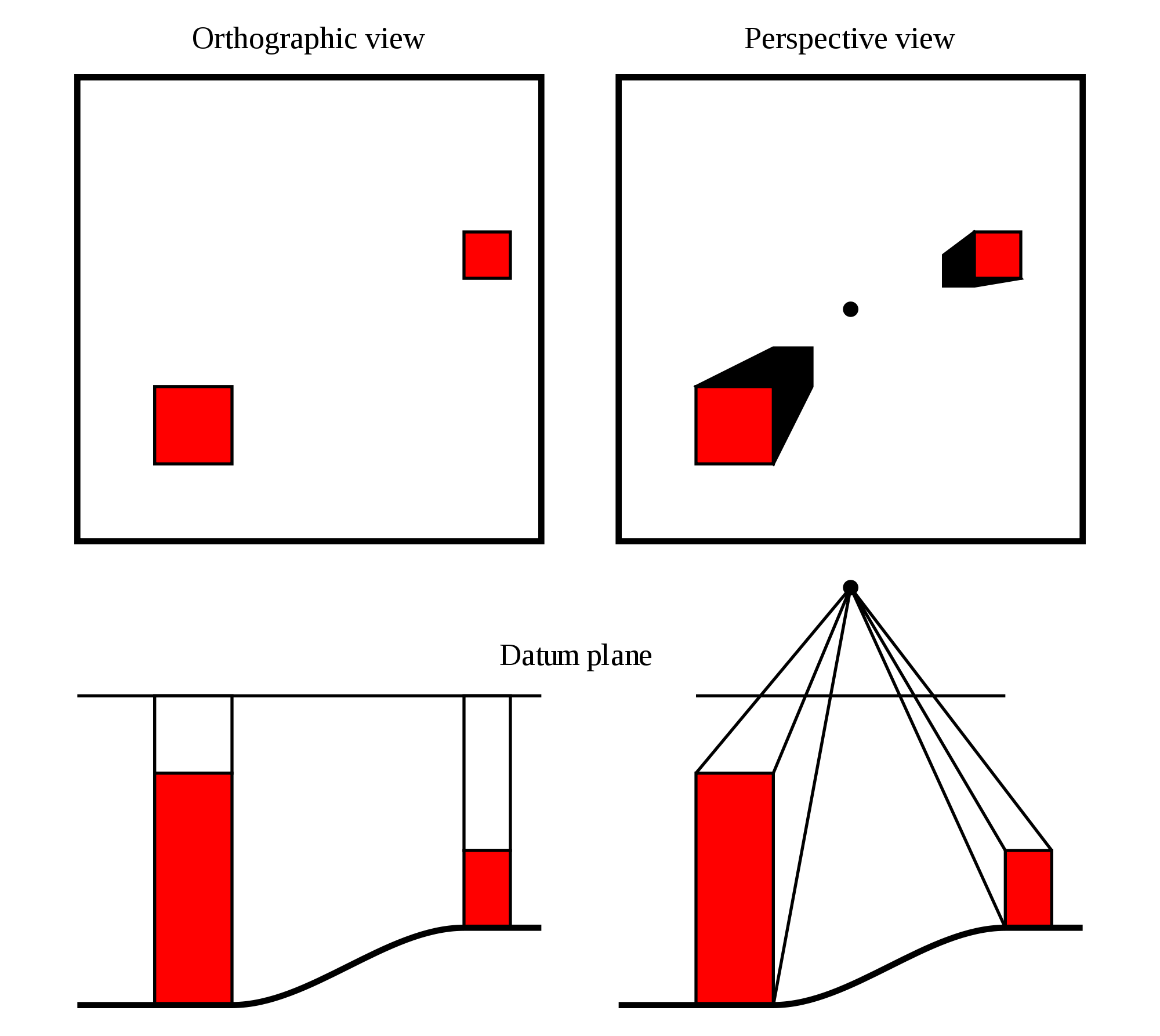
An orthophoto, orthophotograph, orthoimage or orthoimagery is an aerial photograph or satellite imagery geometrically corrected ("orthorectified") such that the scale is uniform: the photo or image follows a given map projection. Unlike an uncorrected aerial photograph, an orthophoto can be used to measure true distances, because it is an accurate representation of the Earth's surface, having been adjusted for topographic relief,[1] lens distortion, and camera tilt.
Orthophotographs are commonly used in geographic information systems (GIS) as a "map accurate" background image. An orthorectified image differs from rubber sheeted rectifications as the latter may accurately locate a number of points on each image but stretch the area between so scale may not be uniform across the image. A digital elevation model (DEM) or topographic map is required to create an orthophoto, as distortions in the image due to the varying distance between the camera/sensor and different points on the ground need to be corrected. An orthoimage and a "rubber sheeted" image can both be said to have been georeferenced; however, the overall accuracy of the rectification varies. Software can display the orthophoto and allow an operator to digitize or place linework, text annotations or geographic symbols (such as hospitals, schools, and fire stations). Some software can process the orthophoto and produce the linework automatically.
Production of orthophotos was historically achieved using opto-mechanical devices.[2]
The orthorectification is not always perfect and has side effect especially for the geometry of high-rise constructions. When using the top-most digital surface model (DSM), instead of the bottom DTM, the resulting product is called a true orthophoto.[3]
Orthophotomosaic and orthophotomap
[edit].jpg)

An orthophotomosaic is a raster image mosaic made by merging or stitching orthophotos. The aerial or satellite photographs have been transformed to correct for perspective so that they appear to have been taken from vertically above at an infinite distance.[4] Google Earth images are of this type.
The document (digital or paper) representing an orthophotomosaic with additional marginal information like a title, north arrow, scale bar and cartographical information is called an orthophotomap or image map. Often these maps show additional point, line or polygon layers (like a traditional map) on top of the orthophotomosaic. A similar document, mostly used for disaster relief, is called a spatiomap.

See also
[edit]References
[edit]- ^ "Digital Orthophotography and GIS". proceedings.esri.com. Retrieved 2025-08-12.
- ^ BBC Tomorrow's World: How maps are corrected and updated using aerial photography and optical machinery. 18 December 1970.
- ^ Neteler, Markus; Mitasova, Helena (2013-04-18). Open Source GIS: A GRASS GIS Approach. Springer Science & Business Media. ISBN 978-1-4757-3578-9. Retrieved 2025-08-05.
- ^ American Congress on Surveying and Mapping, American Society for Photogrammetry and Remote Sensing (1994), Glossary of the Mapping Sciences, American Society of Civil Engineers, p. 370, ISBN 9780784475706
Further reading
[edit]- Bolstad, P., (2005), GIS Fundamentals: A First Text on Geographic Information Systems, Eider Press, White Bear Lake, MN, 2nd ed.
- Demers, Michael N., (1997). Fundamentals of Geographic Information Systems, John Wiley & Sons.
- Fernandez, E.; Garfinkel, R.; Arbiol, R. (May–June 1998). "Mosaicking of Aerial Photographic Maps Via Seams Defined by Bottleneck Shortest Paths". Operations Research. 46 (3): 293–304. doi:10.1287/opre.46.3.293..
- Petrie, G., (1977), Transactions of the Institute of British Geographers: Orthophotomaps New Series, vol. 2, no.1, Contemporary Cartography., pg. 49-70
- Robinson, A.H., Morrison, J.L., Muehrcke, P.C., Kimerling, A.J., Stephen Guptill, (1995) Elements of Cartography: John Wiley & Sons Inc., Canada, 6th ed.
- United States Geological Survey, US Department of Interior, USGS Fact Sheet May 2001 https://erg.usgs.gov/isb/pubs/factsheets/fs05701.html Archived 2008-06-02 at the Wayback Machine
External links
[edit]Orthophoto
View on GrokipediaDefinition and Characteristics
Definition
An orthophoto is an aerial photograph or satellite image that has been geometrically corrected, or orthorectified, to remove distortions caused by terrain relief, camera tilt, lens distortion, and perspective effects.[2] This correction process ensures that the resulting image has a uniform scale throughout, allowing for accurate planimetric measurements—such as distances and areas—directly on the image, equivalent to those obtained from a traditional map.[2] The mathematical basis of an orthophoto involves transforming the original image from a central perspective projection, inherent to the camera's viewpoint, to an orthogonal projection that represents the terrain as if viewed directly from above.[5] This transformation relies on ground control points to establish spatial references and elevation data, typically from a digital elevation model (DEM), to adjust each pixel's position for relief displacements.[2] An orthophoto differs from an orthophotomosaic, which is a composite image formed by combining multiple individual orthophotos to cover a larger area, and from an orthophotomap, which incorporates additional cartographic elements such as contour lines or labels onto the orthophoto base.[2]Key Characteristics
Orthophotos exhibit high planimetric accuracy, where ground features are depicted in their true horizontal positions irrespective of terrain elevation variations, enabling reliable measurements for mapping and geographic information systems (GIS). This accuracy is achieved through geometric corrections that align the imagery to a map projection, meeting positional accuracy standards such as those from the American Society for Photogrammetry and Remote Sensing (ASPRS), where horizontal accuracy is typically within 1-pixel root mean square error (RMSE) for high-quality products.[6] A defining trait of orthophotos is their scale invariance, maintaining a uniform scale across the entire image—commonly 1:24,000 for USGS products—unlike conventional aerial photographs where scale varies due to terrain relief and sensor tilt. This constant scale facilitates direct measurement of distances and areas without additional distortion adjustments.[7][8] Orthophotos integrate the detailed photographic qualities of aerial imagery, such as texture, color, and visual fidelity, with the geometric precision of a map by eliminating distortions like radial displacement from camera orientation. This preservation of visual detail while ensuring positional fidelity makes them versatile for applications requiring both aesthetic and analytical value.[2] The resolution of orthophotos, which determines the level of detail, typically ranges from 0.5 to 2 meters per pixel for aerial-derived sources, influenced by factors such as flight altitude and sensor capabilities; for instance, recent USGS National Agriculture Imagery Program (NAIP) orthophotos achieve 0.6-meter resolution nationally (as of 2025). Orthophotos are commonly stored in GeoTIFF format, which embeds georeferencing information to support integration with spatial data systems like GIS software.[9][10][8]History
Early Concepts
The foundational concepts of orthophotos emerged in the 1930s within the field of photogrammetry, driven by the need to correct distortions in aerial imagery caused by terrain relief displacement. Relief displacement, where features at different elevations appear shifted from their true horizontal positions due to the perspective nature of photographs, had long been recognized as a limitation in mapping from aerial photos. Early photogrammetrists, including Earl Church, explored computational approaches to mitigate these distortions through a series of articles published in the 1930s, laying theoretical groundwork for creating scale-invariant images that could serve as map substitutes.[11] A pivotal advancement came in 1936 with the conceptualization and patenting of the Gallus-Ferber Photorestituteur, the first instrument designed specifically for orthophoto production. Developed by Robert Ferber in France, building on earlier principles outlined by Gallus in 1927–1928, this analog device aimed to project aerial photographs onto a horizontal plane while compensating for relief using elevation data, effectively eliminating both tilt and topographic distortions. Although not widely adopted due to its mechanical complexity and cost, it represented the initial practical attempt to realize distortion-free aerial imagery through opto-mechanical means. Similarly, in the United States, Russell K. Bean independently conceived the orthophotoscope in 1936, envisioning a stereoscopic scanning system to generate uniform-scale orthophotographs, though development was deferred until the 1950s.[12][13] Following World War II, the demand for accurate reconnaissance imagery from military applications spurred further theoretical modeling of orthorectification processes in the 1950s. Advances in photogrammetric instrumentation, influenced by wartime aerial surveying needs, focused on analytical methods to integrate elevation models with photo projections, enabling more precise corrections for relief and tilt. These models emphasized the use of stereo-plotters and profile tracing to simulate terrain-adjusted views, though implementation remained constrained by the era's reliance on manual and analog techniques owing to the absence of digital computing capabilities. This period marked a conceptual bridge toward later practical implementations.[14]Key Milestones
The 1960s marked a period of significant momentum in equipment development for orthophoto production, with the introduction of analog orthophoto plotters that facilitated semi-automated processes. The U.S. Geological Survey (USGS) advanced the orthophoto concept through the development of a practical orthophotoscope, patented in 1959 by Russell K. Bean, which enabled the generation of orthophotoquads as a standard product. Analog production of orthophotos began at the USGS Western Mapping Center in Menlo Park, California, in 1965, using instruments like the T-61 Orthophotoscope.[15][12][13] In the 1970s, orthophoto production began integrating with early computer-assisted photogrammetry, allowing for initial digital rectification methods. These developments enabled the simultaneous creation of orthophotographs and digital elevation models using computational tools.[16][15] The year 1987 saw the USGS introduce the Digital Orthophoto Quadrangle (DOQ) program, which standardized scanned and rectified aerial photographs at a 1:24,000 scale across the contiguous United States and continued production until 2006. This initiative utilized digital scanning of photographic stereo pairs combined with processing software to produce georeferenced imagery.[17][16] From the 1990s through the 2000s, orthophoto workflows transitioned to fully digital systems, bolstered by GIS software such as ARC/INFO, which was launched in 1982 and supported automated processing alongside higher-resolution outputs. The first USGS National Mapping Program Standard for Digital Orthophotos was released in 1992, with major revisions in 1996 to support UTM projections and datums like NAD 83. ARC/INFO's topological data structure became essential for integrating orthophotos into broader GIS applications by the late 1980s.[15][13][18] Since the 2010s, advancements in unmanned aerial vehicles (UAVs) and satellite imagery have lowered production costs and enhanced accessibility for orthophoto generation among non-experts. Following the DOQ program's end, the USGS's National Agriculture Imagery Program (NAIP), part of The National Map, has provided current high-resolution orthoimagery, with cycles every three years as of 2025. UAV photogrammetry evolved rapidly during this decade, enabling high-resolution orthophoto creation through automated image processing pipelines. Concurrent satellite improvements, such as those from Landsat missions, provided more frequent and refined data for orthorectified products.[19][20][21][22]Production Process
Data Acquisition
Data acquisition for orthophotos commences with the collection of raw imagery and ancillary data to ensure geometric fidelity and spectral accuracy in the final product. Primary imagery sources include aerial platforms such as fixed-wing aircraft for broad-area coverage and unmanned aerial vehicles (UAVs) for high-resolution, site-specific surveys, alongside satellite systems like the Landsat series and Sentinel-2 for global-scale multispectral data. Fixed-wing flights provide efficient collection over large regions, while UAVs enable flexible deployment in constrained environments, and satellites offer consistent, repeat-pass observations without on-site logistics.[17][23][24][25] Sensors used in these acquisitions typically consist of digital frame cameras capturing visible and near-infrared bands, with options for multispectral or hyperspectral configurations to record additional wavelengths for enhanced feature discrimination. For traditional aerial photography, large-format metric cameras ensure uniform scale, while modern digital sensors on UAVs and satellites incorporate pushbroom or whiskbroom technologies for continuous scanning. Critical metadata, including precise sensor position, orientation (via inertial measurement units), and focal length parameters, is embedded during capture to support bundle adjustment in processing.[23][23][23] Flight planning for aerial data collection emphasizes systematic coverage to facilitate stereoscopic analysis and seamless mosaicking. Forward overlaps of 60-80% and lateral overlaps of 30-60% (higher for UAVs) between consecutive images are standard to generate sufficient tie points for 3D reconstruction, with higher percentages applied in vegetated or textured-variable terrains. Altitudes are generally set between 500 and 3000 meters above ground level to balance resolution and swath width, yielding ground sample distances suitable for mapping scales from 1:1000 to 1:5000. Ground control points (GCPs) are surveyed using differential GPS receivers at evenly distributed locations across the project area, typically 5-20 points per square kilometer depending on terrain complexity,[26] to anchor the imagery to real-world coordinates. Supporting elevation data, in the form of digital elevation models (DEMs) or digital terrain models (DTMs), is obtained through complementary methods to model relief for later correction. LiDAR systems mounted on aircraft or UAVs deliver dense point clouds by measuring laser pulse returns, achieving vertical accuracies of 10-15 cm over varied topography. Radar interferometry from satellites like those in the TanDEM-X mission provides all-weather DEMs at 12-meter resolution globally, while photogrammetric techniques extract DTMs from overlapping stereo pairs of the primary imagery itself. These elevation datasets must align spatially and temporally with the imagery to minimize discrepancies in orthorectification.[27][28][23] Several quality factors govern the success of data acquisition to mitigate distortions and ensure usability. Favorable atmospheric conditions, such as low humidity and minimal cloud cover below 25%, are essential to reduce haze and scattering effects on image clarity. Acquisitions are timed for early morning or late afternoon to minimize long shadows from structures and terrain features, which can obscure up to 27% of coastal habitats if captured midday. Target resolutions are application-specific, with urban areas often requiring 5 cm per pixel to resolve infrastructure details, while rural surveys may suffice at 20-50 cm. The acquired DEM supports subsequent orthorectification by providing terrain relief data for distortion removal.[29][29][30][23]Orthorectification
Orthorectification is the geometric correction process that transforms perspective-distorted aerial or satellite imagery into a planimetrically accurate orthographic projection by removing displacements caused by terrain relief, sensor orientation, and topographic variations.[31] This involves mathematical resampling of image pixels to their true ground positions using a sensor model, interior and exterior orientation parameters, and a digital elevation model (DEM) to account for elevation differences.[32] The result is an image where every pixel corresponds to a uniform ground scale, enabling direct measurements as on a map.[33] The core of orthorectification relies on the collinearity equations, which ensure that the optical ray from the camera center through the image point aligns with the corresponding ground point. These equations model the transformation from object space coordinates to image coordinates , incorporating the focal length , principal point offsets, and rotation matrix elements derived from orientation parameters. The standard form is: where is the principal point, and is the camera center position.[34] The DEM provides the elevation values to iteratively correct relief displacements, projecting points onto an ellipsoidal surface like WGS84.[34] The process begins with establishing ground control points (GCPs) to refine the sensor model through bundle adjustment, which minimizes errors in orientation parameters by solving the collinearity equations across multiple images or points.[35] Elevations are then interpolated from the DEM for each pixel, enabling the computation of corrected ground coordinates via the collinearity model. Finally, pixels are resampled onto a uniform output grid using methods such as nearest neighbor for categorical data preservation or bilinear interpolation for smoother radiometric continuity.[36] Emerging methods as of 2025 incorporate neural radiance fields (NeRF), such as Ortho-NeRF, to generate true digital orthophotos directly from multi-view UAV images, enhancing efficiency for high-relief terrains without relying solely on traditional DEMs.[37] Common software for orthorectification includes commercial packages like ERDAS IMAGINE, which supports rigorous sensor modeling and automated bundle adjustment for high-resolution imagery, and PCI Geomatica, offering tools for DEM-based correction of satellite data using rational polynomial coefficients.[38][39] Open-source options like GDAL provide efficient command-line utilities, such asgdalwarp, for terrain-corrected rectification with RPC support and DEM integration.[40]
A primary error source in orthorectification is DEM inaccuracies, which introduce residual distortions by misrepresenting terrain heights, leading to positional offsets in the output image. For instance, using a low-resolution DEM derived from 1:50,000-scale maps can result in root mean square errors up to 2.57 meters, equivalent to 1-2 pixels for typical 1-meter resolution orthophotos.[41] Higher-quality DEMs, such as those from 1:10,000-scale sources, reduce these to under 1.55 meters, emphasizing the need for DEM resolution matched to image scale.[42]
Mosaicking and Finalization
After orthorectification, multiple adjacent images are assembled into a seamless mosaic to create a continuous orthophoto coverage. This mosaicking process involves determining optimal seamlines between overlapping images to minimize visual discontinuities, followed by blending techniques such as feathering, where pixel values in overlap regions are weighted averaged to ensure smooth transitions.[43] Histogram matching is often applied prior to feathering to align the tonal distributions of adjacent images, reducing color and brightness differences that could cause noticeable seams.[44] These methods are typically implemented using specialized software that automates seamline detection based on gradient magnitude and image content, ensuring the final mosaic appears as a single, uniform image.[45] Color balancing addresses variations in exposure and illumination across flight lines or different imaging sessions, which can result from atmospheric conditions or sensor inconsistencies. Automated algorithms perform global-to-local adjustments by analyzing histograms or statistical properties of the images and applying corrections to achieve radiometric consistency throughout the mosaic.[46] For instance, tonal balancing may lighten or darken adjacent images during mosaicking to harmonize brightness levels, often using iterative matching processes to refine the overall color profile.[47] This step is crucial for maintaining perceptual uniformity, particularly in large-scale productions where manual intervention would be impractical.[48] The finalized mosaic is then prepared for distribution through tiling, where the large composite is divided into smaller, manageable files for efficient storage and access. Common compressed formats include MrSID, which uses wavelet-based compression to preserve image quality at high ratios, and JPEG2000, supporting lossless or lossy options suitable for geospatial data.[49] Georeferencing is embedded either directly in formats like GeoTIFF or via accompanying world files that define the spatial transformation, with metadata including details such as pixel resolution and acquisition parameters.[50] Quality control ensures the mosaic meets standards for both visual and geometric integrity. Visual inspection identifies artifacts like residual seams, color mismatches, or distortions, often supplemented by automated checks for anomalies.[45] Positional accuracy is quantified using root-mean-square error (RMSE) calculations against ground control points, with targets typically below 1 pixel to achieve sub-pixel precision at the 95% confidence level.[51] These assessments follow guidelines from bodies like the American Society for Photogrammetry and Remote Sensing (ASPRS), confirming the mosaic's reliability for mapping applications.[6] Finally, the orthophoto is assigned a uniform scale and standardized map projection, such as Universal Transverse Mercator (UTM), to facilitate integration with other geospatial datasets. This ensures precise alignment with vector data layers, like boundaries or infrastructure, by maintaining consistent coordinate systems and resolutions.[52] The projection choice, often UTM zones in meters, supports seamless overlay in geographic information systems without additional transformations.[53]Types
True Orthophotos
True orthophotos represent a high-precision variant of orthophotos generated through rigorous photogrammetric techniques, incorporating analytical aerotriangulation and high-accuracy digital surface models (DSMs) to achieve sub-pixel geometric precision across the entire image.[54] Unlike simpler orthorectification methods, true orthophotos utilize DSMs that model both terrain and elevated features such as buildings, ensuring accurate projection and elimination of occlusions or displacements for all visible elements.[54] This approach enables a geometrically complete representation of the Earth's surface in orthographic projection, with every pixel mapped to its true planimetric position.[55] The production of true orthophotos demands stereo aerial imagery to derive detailed DSMs via stereophotogrammetry, complemented by extensive ground control points (GCPs)—typically at least four well-distributed points per block, though higher densities are employed for precision—and bundle block adjustment to simultaneously refine exterior orientation parameters and object coordinates.[56] Analytical aerotriangulation forms the core of this process, solving collinearity equations through least-squares adjustment of image rays, tie points, and GCPs to minimize residuals and achieve robust georeferencing.[56] Additional steps include ray-tracing for occlusion detection and multi-image mosaicking with radiometric balancing to fill gaps and ensure seamless integration.[54] These orthophotos attain positional accuracies with root-mean-square errors (RMSE) below 0.5 meters horizontally, often reaching sub-pixel levels (e.g., 1-2 pixels for 5 cm ground sample distance), rendering them ideal for large-scale mapping at 1:1,000 or finer scales.[6] Such precision supports demanding applications like engineering surveys for infrastructure design and cadastral mapping for legal boundary delineation, where verifiable accuracy is essential.[57][58] However, the heightened complexity of true orthophoto production incurs elevated costs compared to standard digital orthophotos, stemming from requirements for stereo capture, dense DSM generation, manual quality verification of adjustments, and specialized photogrammetric hardware or software for bundle adjustment and occlusion handling.[59][56]Digital Orthophotos
Digital orthophotos are raster-format images derived from either scanned analog aerial photographs or direct digital sensor captures, such as those from satellites or aircraft, where geometric distortions due to terrain relief, sensor tilt, and topography are corrected using mathematical models like polynomial transformations or rational polynomial coefficients (RPCs).[7][60] These models approximate the relationship between image coordinates and ground positions, enabling efficient rectification without requiring full physical sensor parameters.[32] RPCs, in particular, represent this relationship as ratios of cubic polynomials, facilitating automated processing for high-volume satellite data.[61] The production process emphasizes automation and efficiency, utilizing specialized software to perform orthorectification with a limited set of ground control points (GCPs), typically 4-8 per image, which are precisely surveyed locations used to tie the image to real-world coordinates. These GCPs enable the software to solve for transformation parameters, often supplemented by vendor-provided RPC files for satellite imagery.[62] Correction relies on integrating a digital elevation model (DEM) to project each pixel onto a uniform map plane, with coarser resolutions like 10 meters proving sufficient for many applications due to the focus on regional coverage rather than fine detail.[63] This approach contrasts with more intensive methods by minimizing manual intervention and computational demands. Positional accuracy in digital orthophotos typically achieves root-mean-square errors (RMSE) of 1-3 meters horizontally, aligning with standards for regional mapping at scales such as 1:24,000, where features are expected to be within 12.2 meters at 90% confidence per National Map Accuracy Standards (NMAS).[64][63] Such levels support reliable overlay with vector data in geographic information systems, though accuracy can vary based on GCP quality, DEM precision (e.g., RMSE ≤7 meters vertically), and image resolution (often 1 meter ground sample distance).[7] A key advantage of digital orthophotos lies in their accessibility, with production costs reduced through automated workflows and the use of readily available satellite data, as exemplified by the USGS Digital Orthophoto Quadrangles (DOQs), which cover large areas at 1-meter resolution for nationwide mapping.[17] This enables faster turnaround times compared to traditional analog methods, facilitating broad dissemination via public repositories.[63] Despite these benefits, limitations arise in precision, particularly potential distortions at image edges in complex terrain, where simplified polynomial or RPC models may not fully capture varying relief or off-nadir viewing angles, leading to residual displacements up to several pixels.[32] Mosaicking multiple images can mitigate some seam issues but requires careful radiometric balancing.[64]Applications
Cartography and Mapping
Orthophotos play a central role in topographic mapping by serving as geometrically accurate backdrops onto which contours, labels, and symbols are overlaid to produce detailed maps. In the United States, the U.S. Geological Survey (USGS) utilizes digital orthophoto quadrangles (DOQs) as foundational layers for 7.5-minute topographic maps, enabling the integration of elevation data and cultural features to create comprehensive representations of terrain and infrastructure.[17][65] This approach ensures that maps reflect real-world geometry without distortions from camera tilt or terrain relief, providing a reliable visual base for national surveys.[66] The availability of orthophotos facilitates rapid update cycles for topographic maps by incorporating current aerial imagery, which minimizes the reliance on extensive field surveys. For instance, USGS revision programs extract feature updates directly from DOQs and recent photographs, allowing maps to be refreshed efficiently as landscapes change due to development or natural events.[67] Photogrammetric techniques underlying orthophoto production further enhance this efficiency by improving the overall mapping workflow compared to traditional methods.[68] Orthophotos are commonly applied at scales ranging from 1:5,000 to 1:50,000, supporting urban planning and infrastructure projects where precise spatial detail is essential. At these scales, they provide high-resolution bases for mapping settlements, transportation networks, and land use patterns, as seen in projects producing ortho-photographs for urban areas in various regions.[69][70] In hybrid map production, orthophotos are overlaid with vector data such as roads and administrative boundaries to combine photorealistic imagery with schematic elements, resulting in versatile cartographic products.[71][72] Since the 1990s, European national mapping agencies have incorporated orthophotos into official cadastral sheets, enhancing the accuracy and currency of property and land records. For example, France's Institut Géographique National (IGN) integrates orthophotos with cadastral data to produce scaled image maps that support legal and planning documentation.[73] Similarly, the UK's Ordnance Survey has employed orthophoto layers in its MasterMap products for detailed topographic and cadastral applications across urban and rural areas.[74] In recent years, unmanned aerial vehicle (UAV) or drone-based orthophotos have expanded applications in cartography, particularly for high-resolution mapping of small to medium areas. As of 2025, UAV orthophotos are used in heritage site monitoring and infrastructure projects, providing sub-centimeter accuracy for detailed topographic updates without the need for manned flights.[75]Geographic Information Systems
Orthophotos serve as a fundamental base layer in geographic information systems (GIS), providing a geometrically corrected, planimetrically accurate visual reference for overlaying and georeferencing vector data such as roads, boundaries, and infrastructure. This integration enables precise spatial alignment, where orthophotos act as a backdrop for digitizing or verifying vector features, ensuring that positional accuracy is maintained across datasets. In GIS environments, orthophotos facilitate georeferencing by supplying control points derived from their inherent coordinate systems, which are typically aligned to national grids or projected coordinate systems, thereby minimizing distortion in subsequent analyses.[76][77] Beyond basic referencing, orthophotos support advanced feature extraction within GIS workflows, particularly through image processing techniques for automated detection of built environments. For instance, object-based image analysis (OBIA) applied to orthophotos can delineate building footprints by segmenting pixels based on spectral and textural attributes, achieving high accuracy in urban settings where traditional manual digitization is labor-intensive. This process often involves machine learning algorithms, such as convolutional neural networks, to classify and extract features like rooftops from high-resolution orthophotos, integrating seamlessly with GIS for vector output generation.[78][79] In spatial analysis applications, orthophotos enable robust change detection and modeling within GIS, such as monitoring deforestation through multi-temporal comparisons. By differencing pixel values between sequential orthophoto series, analysts can quantify canopy loss or gain, with studies demonstrating over 90% accuracy in identifying deforested areas when combined with GIS overlay tools. Similarly, urban growth modeling utilizes temporal orthophoto sequences to simulate expansion patterns, employing logistic regression or cellular automata in GIS to predict future land use based on historical trends observed in the imagery.[80][81] Orthophotos integrate effectively with popular GIS software like ArcGIS and QGIS, supporting raster-vector overlays for interactive queries and spatial joins. In ArcGIS, orthophotos can be loaded as raster layers for on-the-fly reprojection and analysis with vector data, enabling tools like spatial analyst for buffer operations or zonal statistics. QGIS offers similar compatibility through plugins and native tools for merging orthophotos with shapefiles, facilitating queries on overlaid features such as land parcels. This interoperability enhances data fusion, particularly when orthophotos are combined with multispectral remote sensing data for refined land cover classification; for example, fusing visible-band orthophotos with near-infrared multispectral layers improves supervised classification accuracy to 95% or higher in GIS-based thematic mapping.[82][83][84] Practical examples of orthophoto use in GIS appear in environmental impact assessments, such as those conducted by the U.S. Environmental Protection Agency (EPA) through EnviroAtlas, where orthophotos underpin ecosystem service mapping and habitat change analysis. In European Union projects, tools like the IMPACT Toolbox from the Joint Research Centre leverage orthophotos within GIS for forest monitoring and biodiversity assessments, integrating them to evaluate impacts from land development. These applications demonstrate how orthophotos enhance decision-making by providing verifiable, high-resolution evidence for policy and planning.[85][86] UAV-derived orthophotos have gained prominence in GIS applications as of 2025, enabling rapid data collection for dynamic monitoring tasks such as trail condition assessment and urban landscape changes. Integrated with GIS platforms like Google Earth Engine, they support high-resolution impervious surface mapping and disaster management, offering flexibility for site-specific analyses.[87][88][89]Advantages and Limitations
Advantages
Orthophotos enable precise measurements of distances and areas directly from the imagery, eliminating the need for on-site field visits in many cases. High-quality orthophotos can achieve sub-meter positional accuracy (e.g., RMSE < 1 m), allowing reliable geometric calculations comparable to traditional maps.[90][91] Unlike line-drawn maps, orthophotos preserve the photographic realism of aerial imagery, including natural colors, textures, and fine details of terrain and features. This visual fidelity provides an intuitive and detailed representation that enhances interpretability for users in planning and analysis.[90] Orthophotos support timely updates through repeat aerial acquisitions, facilitating rapid monitoring of changes such as urban development or environmental shifts. In disaster response scenarios, they deliver quick, accurate data for assessment and planning, often faster than satellite alternatives under optimal conditions. Recent AI techniques, such as neural radiance fields (NeRF), further enhance processing speed and fidelity for complex environments.[93][94][95] The production of orthophotos is cost-effective, particularly with digital processing methods that minimize reliance on extensive ground surveys and fieldwork. This efficiency reduces overall expenses while maintaining high utility across diverse applications.[96][91] Orthophotos exhibit versatility in scale, applicable from local drone-based surveys covering small sites to broad satellite-derived coverage for regional or global extents. This adaptability makes them suitable for a wide range of spatial resolutions and project sizes.[97][98]Limitations
The accuracy of orthophotos heavily depends on the quality of the underlying digital elevation model (DEM), as inaccuracies in elevation data lead to residual relief displacement, particularly in areas with varying topography. However, emerging AI-based methods like 3D Gaussian Splatting reduce DEM dependency for true orthophotos in urban settings.[99][100] In hilly or mountainous regions, such errors can result in positional displacements of 5-10 meters or more for a significant portion of pixels, with maximum deviations reaching up to 60 meters in steep terrain when using lower-resolution DEMs like 90-meter PlanetDEM.[99] These distortions arise because orthorectification fails to fully correct for terrain-induced shifts without precise elevation information, compromising the planimetric fidelity of the final product.[99] Orthophoto production is computationally intensive, demanding substantial hardware resources for processing large areas, and often time-consuming when relying on manual ground control points (GCPs) for georeferencing.[101] Software like Agisoft Metashape, commonly used for orthophoto generation, requires 64-128 GB of RAM and professional GPUs with 24+ GB VRAM for projects involving 1000+ high-resolution images covering extensive regions.[101] Manual GCP placement, essential for accurate bundle adjustment in areas with limited automatic tie points, can extend processing times significantly, making it impractical for real-time or very large-scale applications without automation.[102] Cost barriers further limit the accessibility of true orthophotos, with production expenses typically ranging from $10 to $50 per square kilometer depending on resolution, archive status, and stereo capabilities (as of 2024).[103] High-resolution (30-50 cm) orthorectified imagery from providers like Maxar or Airbus can cost up to $65 per km² for new acquisitions, which restricts widespread adoption in developing regions where budgets for geospatial data are constrained.[103] Temporal factors, such as shadows, vegetation changes, and seasonal variations, can degrade the interpretability of orthophotos by introducing inconsistencies in image tone and feature visibility.[79] Shadows from trees or structures obscure underlying details, leading to incomplete feature extraction and reduced accuracy in analyses like building footprint delineation, while seasonal shifts in vegetation density—such as leaf-on conditions in summer versus sparse growth in early spring—alter spectral signatures and complicate object discrimination.[79] Orthophotos are inherently limited by their pixel resolution, preventing the capture of sub-pixel details and rendering them unsuitable for identifying very small features without ultra-high-resolution source imagery.[104] At a ground sample distance (GSD) of 15 cm, for instance, objects smaller than 15x15 cm blend into surrounding pixels, losing distinctiveness; finer details require sub-30 cm resolutions typically obtained from aerial platforms rather than standard satellite sources.[104]References
- https://www.usgs.gov/centers/eros/science/usgs-eros-archive-aerial-photography-national-agriculture-[imagery](/page/Imagery)-program-naip