
Community hub
Recent from talks
Contribute something
Nothing was collected or created yet.
Pre- and post-test probability
View on WikipediaPre-test probability and post-test probability (alternatively spelled pretest and posttest probability) are the probabilities of the presence of a condition (such as a disease) before and after a diagnostic test, respectively. Post-test probability, in turn, can be positive or negative, depending on whether the test falls out as a positive test or a negative test, respectively. In some cases, it is used for the probability of developing the condition of interest in the future.
Test, in this sense, can refer to any medical test (but usually in the sense of diagnostic tests), and in a broad sense also including questions and even assumptions (such as assuming that the target individual is a female or male). The ability to make a difference between pre- and post-test probabilities of various conditions is a major factor in the indication of medical tests.
Pre-test probability
[edit]The pre-test probability of an individual can be chosen as one of the following:
- The prevalence of the disease, which may have to be chosen if no other characteristic is known for the individual, or it can be chosen for ease of calculation even if other characteristics are known although such omission may cause inaccurate results
- The post-test probability of the condition resulting from one or more preceding tests
- A rough estimation, which may have to be chosen if more systematic approaches are not possible or efficient
Estimation of post-test probability
[edit]In clinical practice, post-test probabilities are often just estimated or even guessed. This is usually acceptable in the finding of a pathognomonic sign or symptom, in which case it is almost certain that the target condition is present; or in the absence of finding a sine qua non sign or symptom, in which case it is almost certain that the target condition is absent.
In reality, however, the subjective probability of the presence of a condition is never exactly 0 or 100%. Yet, there are several systematic methods to estimate that probability. Such methods are usually based on previously having performed the test on a reference group in which the presence or absence on the condition is known (or at least estimated by another test that is considered highly accurate, such as by "Gold standard"), in order to establish data of test performance. These data are subsequently used to interpret the test result of any individual tested by the method. An alternative or complement to reference group-based methods is comparing a test result to a previous test on the same individual, which is more common in tests for monitoring.
The most important systematic reference group-based methods to estimate post-test probability includes the ones summarized and compared in the following table, and further described in individual sections below.
| Method | Establishment of performance data | Method of individual interpretation | Ability to accurately interpret subsequent tests | Additional advantages |
|---|---|---|---|---|
| By predictive values | Direct quotients from reference group | Most straightforward: Predictive value equals probability | Usually low: Separate reference group required for every subsequent pre-test state | Available both for binary and continuous values |
| By likelihood ratio | Derived from sensitivity and specificity | Post-test odds given by multiplying pretest odds with the ratio | Theoretically limitless | Pre-test state (and thus the pre-test probability) does not have to be same as in reference group |
| By relative risk | Quotient of risk among exposed and risk among unexposed | Pre-test probability multiplied by the relative risk | Low, unless subsequent relative risks are derived from same multivariate regression analysis | Relatively intuitive to use |
| By diagnostic criteria and clinical prediction rules | Variable, but usually most tedious | Variable | Usually excellent for all test included in criteria | Usually most preferable if available |
By predictive values
[edit]Predictive values can be used to estimate the post-test probability of an individual if the pre-test probability of the individual can be assumed roughly equal to the prevalence in a reference group on which both test results and knowledge on the presence or absence of the condition (for example a disease, such as may determined by "Gold standard") are available.
If the test result is of a binary classification into either positive or negative tests, then the following table can be made:
| Condition (as determined by "Gold standard") |
||||
| Positive | Negative | |||
| Test outcome |
Positive | True Positive | False Positive (Type I error) |
→ Positive predictive value |
| Negative | False Negative (Type II error) |
True Negative | → Negative predictive value | |
| ↓ Sensitivity |
↓ Specificity |
↘ Accuracy | ||
Pre-test probability can be calculated from the diagram as follows:
Pretest probability = (True positive + False negative) / Total sample
Also, in this case, the positive post-test probability (the probability of having the target condition if the test falls out positive), is numerically equal to the positive predictive value, and the negative post-test probability (the probability of having the target condition if the test falls out negative) is numerically complementary to the negative predictive value ([negative post-test probability] = 1 - [negative predictive value]),[1] again assuming that the individual being tested does not have any other risk factors that result in that individual having a different pre-test probability than the reference group used to establish the positive and negative predictive values of the test.
In the diagram above, this positive post-test probability, that is, the posttest probability of a target condition given a positive test result, is calculated as:
Positive posttest probability = True positives / (True positives + False positives)
Similarly:
The post-test probability of disease given a negative result is calculated as:
Negative posttest probability = 1 - (True negatives / (False negatives + True negatives))
The validity of the equations above also depend on that the sample from the population does not have substantial sampling bias that make the groups of those who have the condition and those who do not substantially disproportionate from corresponding prevalence and "non-prevalence" in the population. In effect, the equations above are not valid with merely a case-control study that separately collects one group with the condition and one group without it.
By likelihood ratio
[edit]The above methods are inappropriate to use if the pretest probability differs from the prevalence in the reference group used to establish, among others, the positive predictive value of the test. Such difference can occur if another test preceded, or the person involved in the diagnostics considers that another pretest probability must be used because of knowledge of, for example, specific complaints, other elements of a medical history, signs in a physical examination, either by calculating on each finding as a test in itself with its own sensitivity and specificity, or at least making a rough estimation of the individual pre-test probability.
In these cases, the prevalence in the reference group is not completely accurate in representing the pre-test probability of the individual, and, consequently, the predictive value (whether positive or negative) is not completely accurate in representing the post-test probability of the individual of having the target condition.
In these cases, a posttest probability can be estimated more accurately by using a likelihood ratio for the test. Likelihood ratio is calculated from sensitivity and specificity of the test, and thereby it does not depend on prevalence in the reference group,[2] and, likewise, it does not change with changed pre-test probability, in contrast to positive or negative predictive values (which would change). Also, in effect, the validity of post-test probability determined from likelihood ratio is not vulnerable to sampling bias in regard to those with and without the condition in the population sample, and can be done as a case-control study that separately gathers those with and without the condition.
Estimation of post-test probability from pre-test probability and likelihood ratio goes as follows:[2]
- Pretest odds = Pretest probability / (1 - Pretest probability)
- Posttest odds = Pretest odds * Likelihood ratio
In equation above, positive post-test probability is calculated using the likelihood ratio positive, and the negative post-test probability is calculated using the likelihood ratio negative.
- Posttest probability = Posttest odds / (Posttest odds + 1)

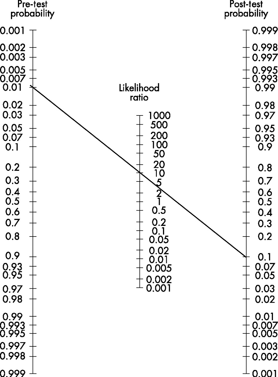
The relation can also be estimated by a so-called Fagan nomogram (shown at right) by making a straight line from the point of the given pre-test probability to the given likelihood ratio in their scales, which, in turn, estimates the post-test probability at the point where that straight line crosses its scale.
The post-test probability can, in turn, be used as pre-test probability for additional tests if it continues to be calculated in the same manner.[2]
-
 Diagram relating pre- and post-test probabilities, with the green curve (upper left half) representing a positive test, and the red curve (lower right half) representing a negative test, for the case of 90% sensitivity and 90% specificity, corresponding to a likelihood ratio positive of 9, and a likelihood ratio negative of 0.111. The length of the green arrows represent the change in absolute (rather than relative) probability given a positive test, and the red arrows represent the change in absolute probability given a negative test.
It can be seen from the length of the arrows that, at low pre-test probabilities, a positive test gives a greater change in absolute probability than a negative test (a property that is generally valid as long as the specificity isn't much higher than the sensitivity). Similarly, at high pre-test probabilities, a negative test gives a greater change in absolute probability than a positive test (a property that is generally valid as long as the sensitivity isn't much higher than the specificity). -
 Relation between pre-and post-test probabilities for various likelihood ratio positives (upper left half) and various likelihood ratio negatives (lower right half).


It is possible to do a calculation of likelihood ratios for tests with continuous values or more than two outcomes which is similar to the calculation for dichotomous outcomes. For this purpose, a separate likelihood ratio is calculated for every level of test result and is called interval or stratum specific likelihood ratios.[4]
Example
[edit]An individual was screened with the test of fecal occult blood (FOB) to estimate the probability for that person having the target condition of bowel cancer, and it fell out positive (blood were detected in stool). Before the test, that individual had a pre-test probability of having bowel cancer of, for example, 3% (0.03), as could have been estimated by evaluation of, for example, the medical history, examination and previous tests of that individual.
The sensitivity, specificity etc. of the FOB test were established with a population sample of 203 people (without such heredity), and fell out as follows:
| Patients with bowel cancer (as confirmed on endoscopy) |
||||
| Positive | Negative | |||
| Fecal occult blood screen test outcome |
Positive | TP = 2 | FP = 18 | → Positive predictive value = TP / (TP + FP) = 2 / (2 + 18) = 2 / 20 = 10% |
| Negative | FN = 1 | TN = 182 | → Negative predictive value = TN / (FN + TN) = 182 / (1 + 182) = 182 / 183 ≈ 99.5% | |
| ↓ Sensitivity = TP / (TP + FN) = 2 / (2 + 1) = 2 / 3 ≈ 66.67% |
↓ Specificity = TN / (FP + TN) = 182 / (18 + 182) = 182 / 200 = 91% |
↘ Accuracy = (TP + TN) / Total = (2 + 182) / 203 = 184 / 203 = 90.64% | ||
From this, the likelihood ratios of the test can be established:[2]
- Likelihood ratio positive = sensitivity / (1 − specificity) = 66.67% / (1 − 91%) = 7.4
- Likelihood ratio negative = (1 − sensitivity) / specificity = (1 − 66.67%) / 91% = 0.37
- Pretest probability (in this example) = 0.03
- Pretest odds = 0.03 / (1 - 0.03) = 0.0309
- Positive posttest odds = 0.0309 * 7.4 = 0.229
- Positive posttest probability = 0.229 / (0.229 + 1) = 0.186 or 18.6%
Thus, that individual has a post-test probability (or "post-test risk") of 18.6% of having bowel cancer.
The prevalence in the population sample is calculated to be:
- Prevalence = (2 + 1) / 203 = 0.0148 or 1.48%
The individual's pre-test probability was more than twice that of the population sample, although the individual's post-test probability was less than twice that of the population sample (which is estimated by the positive predictive value of the test of 10%), opposite to what would result by a less accurate method of simply multiplying relative risks.
Specific sources of inaccuracy
[edit]Specific sources of inaccuracy when using likelihood ratio to determine a post-test probability include interference with determinants or previous tests or overlap of test targets, as explained below:
Interference with test
[edit]Post-test probability, as estimated from the pre-test probability with likelihood ratio, should be handled with caution in individuals with other determinants (such as risk factors) than the general population, as well as in individuals that have undergone previous tests, because such determinants or tests may also influence the test itself in unpredictive ways, still causing inaccurate results. An example with the risk factor of obesity is that additional abdominal fat can make it difficult to palpate abdominal organs and decrease the resolution of abdominal ultrasonography, and similarly, remnant barium contrast from a previous radiography can interfere with subsequent abdominal examinations,[5] in effect decreasing the sensitivities and specificities of such subsequent tests. On the other hand, the effect of interference can potentially improve the efficacy of subsequent tests as compared to usage in the reference group, such as some abdominal examinations being easier when performed on underweight people.
Overlap of tests
[edit]Furthermore, the validity of calculations upon any pre-test probability that itself is derived from a previous test depend on that the two tests do not significantly overlap in regard to the target parameter being tested, such as blood tests of substances belonging to one and the same deranged metabolic pathway. An example of the extreme of such an overlap is where the sensitivity and specificity has been established for a blood test detecting "substance X", and likewise for one detecting "substance Y". If, in fact, "substance X" and "substance Y" are one and the same substance, then, making a two consecutive tests of one and the same substance may not have any diagnostic value at all, although the calculation appears to show a difference. In contrast to interference as described above, increasing overlap of tests only decreases their efficacy. In the medical setting, diagnostic validity is increased by combining tests of different modalities to avoid substantial overlap, for example in making a combination of a blood test, a biopsy and radiograph.
Methods to overcome inaccuracy
[edit]To avoid such sources of inaccuracy by using likelihood ratios, the optimal method would be to gather a large reference group of equivalent individuals, in order to establish separate predictive values for use of the test in such individuals. However, with more knowledge of an individual's medical history, physical examination and previous test etc. that individual becomes more differentiated, with increasing difficulty to find a reference group to establish tailored predictive values, making an estimation of post-test probability by predictive values invalid.
Another method to overcome such inaccuracies is by evaluating the test result in the context of diagnostic criteria, as described in the next section.
By relative risk
[edit]Post-test probability can sometimes be estimated by multiplying the pre-test probability with a relative risk given by the test. In clinical practice, this is usually applied in evaluation of a medical history of an individual, where the "test" usually is a question (or even assumption) regarding various risk factors, for example, sex, tobacco smoking or weight, but it can potentially be a substantial test such as putting the individual on a weighing scale. When using relative risks, the resultant probability is usually rather related to the individual developing the condition over a period of time (similarly to the incidence in a population), instead of being the probability of an individual of having the condition in the present, but can indirectly be an estimation of the latter.
Usage of hazard ratio can be used somewhat similarly to relative risk.
One risk factor
[edit]To establish a relative risk, the risk in an exposed group is divided by the risk in an unexposed group.
If only one risk factor of an individual is taken into account, the post-test probability can be estimated by multiplying the relative risk with the risk in the control group. The control group usually represents the unexposed population, but if a very low fraction of the population is exposed, then the prevalence in the general population can often be assumed equal to the prevalence in the control group. In such cases, the post-test probability can be estimated by multiplying the relative risk with the risk in the general population.
For example, the incidence of breast cancer in a woman in the United Kingdom at age 55 to 59 is estimated at 280 cases per 100.000 per year,[6] and the risk factor of having been exposed to high-dose ionizing radiation to the chest (for example, as treatments for other cancers) confers a relative risk of breast cancer between 2.1 and 4.0,[7] compared to unexposed. Because a low fraction of the population is exposed, the prevalence in the unexposed population can be assumed equal to the prevalence in the general population. Subsequently, it can be estimated that a woman in the United Kingdom that is aged between 55 and 59 and that has been exposed to high-dose ionizing radiation should have a risk of developing breast cancer over a period of one year of between 588 and 1.120 in 100.000 (that is, between 0,6% and 1.1%).
Multiple risk factors
[edit]Theoretically, the total risk in the presence of multiple risk factors can be estimated by multiplying with each relative risk, but is generally much less accurate than using likelihood ratios, and is usually done only because it is much easier to perform when only relative risks are given, compared to, for example, converting the source data to sensitivities and specificities and calculate by likelihood ratios. Likewise, relative risks are often given instead of likelihood ratios in the literature because the former is more intuitive. Sources of inaccuracy of multiplying relative risks include:
- Relative risks are affected by the prevalence of the condition in the reference group (in contrast to likelihood ratios, which are not), and this issue results in that the validity of post-test probabilities become less valid with increasing difference between the prevalence in the reference group and the pre-test probability for any individual. Any known risk factor or previous test of an individual almost always confers such a difference, decreasing the validity of using relative risks in estimating the total effect of multiple risk factors or tests. Most physicians do not appropriately take such differences in prevalence into account when interpreting test results, which may cause unnecessary testing and diagnostic errors.[8]
- A separate source of inaccuracy of multiplying several relative risks, considering only positive tests, is that it tends to overestimate the total risk as compared to using likelihood ratios. This overestimation can be explained by the inability of the method to compensate for the fact that the total risk cannot be more than 100%. This overestimation is rather small for small risks, but becomes higher for higher values. For example, the risk of developing breast cancer at an age younger than 40 years in women in the United Kingdom can be estimated at 2%.[9] Also, studies on Ashkenazi Jews has indicated that a mutation in BRCA1 confers a relative risk of 21.6 of developing breast cancer in women under 40 years of age, and a mutation in BRCA2 confers a relative risk of 3.3 of developing breast cancer in women under 40 years of age.[10] From these data, it may be estimated that a woman with a BRCA1 mutation would have a risk of approximately 40% of developing breast cancer at an age younger than 40 years, and woman with a BRCA2 mutation would have a risk of approximately 6%. However, in the rather improbable situation of having both a BRCA1 and a BRCA2 mutation, simply multiplying with both relative risks would result in a risk of over 140% of developing breast cancer before 40 years of age, which can not possibly be accurate in reality.
The (latter mentioned) effect of overestimation can be compensated for by converting risks to odds, and relative risks to odds ratios. However, this does not compensate for (former mentioned) effect of any difference between pre-test probability of an individual and the prevalence in the reference group.
A method to compensate for both sources of inaccuracy above is to establish the relative risks by multivariate regression analysis. However, to retain its validity, relative risks established as such must be multiplied with all the other risk factors in the same regression analysis, and without any addition of other factors beyond the regression analysis.
In addition, multiplying multiple relative risks has the same risk of missing important overlaps of the included risk factors, similarly to when using likelihood ratios. Also, different risk factors can act in synergy, with the result that, for example, two factors that both individually have a relative risk of 2 have a total relative risk of 6 when both are present, or can inhibit each other, somewhat similarly to the interference described for using likelihood ratios.
By diagnostic criteria and clinical prediction rules
[edit]Most major diseases have established diagnostic criteria and/or clinical prediction rules. The establishment of diagnostic criteria or clinical prediction rules consists of a comprehensive evaluation of many tests that are considered important in estimating the probability of a condition of interest, sometimes also including how to divide it into subgroups, and when and how to treat the condition. Such establishment can include usage of predictive values, likelihood ratios as well as relative risks.
For example, the ACR criteria for systemic lupus erythematosus defines the diagnosis as presence of at least 4 out of 11 findings, each of which can be regarded as a target value of a test with its own sensitivity and specificity. In this case, there has been evaluation of the tests for these target parameters when used in combination in regard to, for example, interference between them and overlap of target parameters, thereby striving to avoid inaccuracies that could otherwise arise if attempting to calculate the probability of the disease using likelihood ratios of the individual tests. Therefore, if diagnostic criteria have been established for a condition, it is generally most appropriate to interpret any post-test probability for that condition in the context of these criteria.
Also, there are risk assessment tools for estimating the combined risk of several risk factors, such as the online tool [1] from the Framingham Heart Study for estimating the risk for coronary heart disease outcomes using multiple risk factors, including age, gender, blood lipids, blood pressure and smoking, being much more accurate than multiplying the individual relative risks of each risk factor.
Still, an experienced physician may estimate the post-test probability (and the actions it motivates) by a broad consideration including criteria and rules in addition to other methods described previously, including both individual risk factors and the performances of tests that have been carried out.
Clinical use of pre- and post-test probabilities
[edit]A clinically useful parameter is the absolute (rather than relative, and not negative) difference between pre- and post-test probability, calculated as:
Absolute difference = | (pre-test probability) - (post-test probability) |
A major factor for such an absolute difference is the power of the test itself, such as can be described in terms of, for example, sensitivity and specificity or likelihood ratio. Another factor is the pre-test probability, with a lower pre-test probability resulting in a lower absolute difference, with the consequence that even very powerful tests achieve a low absolute difference for very unlikely conditions in an individual (such as rare diseases in the absence of any other indicating sign), but on the other hand, that even tests with low power can make a great difference for highly suspected conditions.
The probabilities in this sense may also need to be considered in context of conditions that are not primary targets of the test, such as profile-relative probabilities in a differential diagnostic procedure.
The absolute difference can be put in relation to the benefit for an individual that a medical test achieves, such as can roughly be estimated as:
, where:

- bn is the net benefit of performing a medical test
- Λp is the absolute difference between pre- and posttest probability of conditions (such as diseases) that the test is expected to achieve.
- ri is the rate of how much probability differences are expected to result in changes in interventions (such as a change from "no treatment" to "administration of low-dose medical treatment").
- bi is the benefit of changes in interventions for the individual
- hi is the harm of changes in interventions for the individual, such as side effects of medical treatment
- ht is the harm caused by the test itself
In this formula, what constitutes benefit or harm largely varies by personal and cultural values, but general conclusions can still be drawn. For example, if the only expected effect of a medical test is to make one disease more likely than another, but the two diseases have the same treatment (or neither can be treated), then ri = 0 and the test is essentially without any benefit for the individual.
Additional factors that influence a decision whether a medical test should be performed or not include: cost of the test, availability of additional tests, potential interference with subsequent test (such as an abdominal palpation potentially inducing intestinal activity whose sounds interfere with a subsequent abdominal auscultation), time taken for the test or other practical or administrative aspects. Also, even if not beneficial for the individual being tested, the results may be useful for the establishment of statistics in order to improve health care for other individuals.
Subjectivity
[edit]Pre- and post-test probabilities are subjective based on the fact that, in reality, an individual either has the condition or not (with the probability always being 100%), so pre- and post-test probabilities for individuals can rather be regarded as psychological phenomena in the minds of those involved in the diagnostics at hand.
See also
[edit]- Diagnostic test interpretation, including general sources of inaccuracy and imprecision
References
[edit]- ^ Evidence-Based Practice Online Course By Mark Ebell. College of Public Health, University of Georgia. Retrieved Aug 2011
- ^ a b c d Likelihood Ratios Archived 22 December 2010 at the Wayback Machine, from CEBM (Centre for Evidence-Based Medicine). Page last edited: 1 February 2009. When used in examples, the general formulas are taken from reference, while example numbers are different
- ^ Parameters taken from image in: Zhang W, Doherty M, Pascual E, et al. (October 2006). "EULAR evidence based recommendations for gout. Part I: Diagnosis. Report of a task force of the Standing Committee for International Clinical Studies Including Therapeutics (ESCISIT)". Ann. Rheum. Dis. 65 (10): 1301–11. doi:10.1136/ard.2006.055251. PMC 1798330. PMID 16707533.
- ^ Brown MD, Reeves MJ (2003). "Evidence-based emergency medicine/skills for evidence-based emergency care. Interval likelihood ratios: another advantage for the evidence-based diagnostician". Ann Emerg Med. 42 (2): 292–297. doi:10.1067/mem.2003.274. PMID 12883521.
- ^ Page 750 (Chapter 10) in: Dunning, Marshall Barnett; Fischbach, Frances Talaska (2009). A manual of laboratory and diagnostic tests [electronic resource]. Philadelphia: Wolters Kluwer Health/Lippincott Williams & Wilkins. ISBN 978-0-7817-7194-8.
- ^ Excel chart for Figure 1.1: Breast Cancer (C50), Average Number of New Cases per Year and Age-Specific Incidence Rates, UK, 2006-2008 at Breast cancer – UK incidence statistics Archived 14 May 2012 at the Wayback Machine at Cancer Research UK. Section updated 18 July 2011.
- ^ ACS (2005). "Breast Cancer Facts & Figures 2005–2006" (PDF). Archived from the original (PDF) on 13 June 2007. Retrieved 26 April 2007.
- ^ Agoritsas, T.; Courvoisier, D. S.; Combescure, C.; Deom, M.; Perneger, T. V. (2010). "Does Prevalence Matter to Physicians in Estimating Post-test Probability of Disease? A Randomized Trial". Journal of General Internal Medicine. 26 (4): 373–378. doi:10.1007/s11606-010-1540-5. PMC 3055966. PMID 21053091.
- ^ 2% given from a cumulative incidence 2.075 cases per 100.000 in females younger up to age 39, from the Cancer Research UK reference above.
- ^ Satagopan, J. M.; Offit, K.; Foulkes, W.; Robson, M. E.; Wacholder, S.; Eng, C. M.; Karp, S. E.; Begg, C. B. (2001). "The lifetime risks of breast cancer in Ashkenazi Jewish carriers of BRCA1 and BRCA2 mutations". Cancer Epidemiology, Biomarkers & Prevention. 10 (5): 467–473. PMID 11352856.