Community hub
Quantitative geography
View on WikipediaQuantitative geography is a subfield and methodological approach to geography that develops, tests, and uses scientific, mathematical, and statistical methods to analyze and model geographic phenomena and patterns.[1][2][3] It aims to explain and predict the distribution and dynamics of human and physical geography through the collection and analysis of quantifiable data.[4] The approach quantitative geographers take is generally in line with the scientific method, where a falsifiable hypothesis is generated, and then tested through observational studies.[3][5][6][7] This has received criticism, and in recent years, quantitative geography has moved to include systematic model creation and understanding the limits of their models.[6][8][9] This approach is used to study a wide range of topics, including population demographics, urbanization, environmental patterns, and the spatial distribution of economic activity.[1] The methods of quantitative geography are often contrasted by those employed by qualitative geography, which is more focused on observing and recording characteristics of geographic place. However, there is increasing interest in using combinations of both qualitative and quantitative methods through mixed-methods research to better understand and contextualize geographic phenomena.[10]
History
[edit]Quantitative geography emerged in the mid-20th century as a response to the increasing demand for more systematic, empirical, and data-driven approaches to studying geographic phenomena.[6] It is a direct product of the quantitative revolution in geography.[1][11]
It was influenced by developments in statistics, mathematics, computer science, and the physical sciences.[12] Quantitative geographers sought to use mathematical and statistical methods to better understand patterns, relationships, and processes in the spatial distribution of human and physical phenomena.
Computers perhaps had the most profound impact on quantitative geography, with techniques such as map analysis, regression analysis, and spatial statistics to investigate various geographic questions.[1] In the 1950s and 1960s, advances in computer technology facilitated the application of quantitative methods in geography, leading to new techniques such as geographic information systems (GIS).[13][14] Notable early pioneers in GIS are Roger Tomlinson and Waldo Tobler.[12] Simultaneously, new data sources, such as remote sensing and GPS, were incorporated into geographic research.[15][16] These tools enabled geographers to collect, analyze, and visualize large amounts of spatial data in new ways, further advancing the field of quantitative geography.[1]
In the late 20th century, quantitative geography became a central discipline within geography, and its influence was felt in fields such as urban, economic, and environmental geography.[1] Within academia, groups such as the Royal Geographical Society Study Group in Quantitative Methods focused on spreading these methods to students and the public through publications such as the Concepts and Techniques in Modern Geography series.[17][18] Economics and spatial econometrics both served as a driving force and area of application for quantitative geography.[19]
Today, research in quantitative geography continues, focusing on using innovative quantitative methods and technologies to address complex geographic questions and problems.
Techniques and subfields
[edit]- Quantitative geography can be divided into many broad categories, such as:
-

-

-

-
-

-


Quantitative revolution
[edit]Laws of geography
[edit]
The concept of laws in geography is a product of the quantitative revolution and is a central focus of quantitative geography.[24] Their emergence is highly influential and one of the major contributions of quantitative geography to the broader branch of technical geography.[25] The discipline of geography is unlikely to settle the matter anytime soon. Several laws have been proposed, and Tobler's first law of geography is the most widely accepted. The first law of geography, and its relation to spatial autocorrelation, is highly influential in the development of technical geography.[25]
Some have argued that geographic laws do not need to be numbered. The existence of a first invites a second, and many are proposed as that. It has also been proposed that Tobler's first law of geography should be moved to the second and replaced with another.[26] A few of the proposed laws of geography are below:
- Tobler's first law of geography: "Everything is related to everything else, but near things are more related than distant"[13][27][26]
- Tobler's second law of geography: "The phenomenon external to a geographic area of interest affects what goes on inside."[27]
- Arbia's law of geography: "Everything is related to everything else, but things observed at a coarse spatial resolution are more related than things observed at a finer resolution."[27][28][29]
- Uncertainty principle: "that the geographic world is infinitely complex and that any representation must therefore contain elements of uncertainty, that many definitions used in acquiring geographic data contain elements of vagueness, and that it is impossible to measure location on the Earth's surface exactly."[26]
Criticism
[edit]This section needs additional citations for verification. (October 2023) |
Critical geography presents critiques against the approach adopted in quantitative geography, sometimes labeled by the critics as a "positivist" approach particularly in relation to the so-called "quantitative revolution" of the 1960s. One of the primary criticisms is reductionism, contending that the emphasis on quantifying data and utilizing mathematical models tends to oversimplify the intricate nature of social and spatial phenomena.[3] Critics also argue that quantitative methods may disregard the unique cultural and historical contexts of specific geographical locations. Critics have likewise argued that reliance on digital mapping tools and technology can restrict the capacity to address certain complex geographical issues and claim that quantitative data collection methods can introduce partiality into the analysis; for example, existing power structures can influence quantitative research by shaping the types of data collected and analyzed.
Quantitative geography has been criticized as being limited in scope because spatial data may not adequately capture certain dimensions of cultural, political, and social relations in human geographies. Lastly, critics emphasize the absence of a critical perspective within this approach, arguing that the unwavering focus on objective and empirical data analysis can divert attention from vital social and political questions, hindering a holistic understanding of geographical issues. The critics argue that these criticisms collectively suggest the need for a more nuanced and context-aware approach in the field of geography.
Response
[edit]Quantitative geographers have responded to the criticisms to various degrees, including that the critiques' broad brush and associated labeling are misplaced.
"Quantitative geographers do not often concern themselves with philosophy, and although externally we are often labeled (incorrectly in many cases) as positivists, such a label has little or zero impact on the way in which we prosecute research. We do not, for example, concern ourselves with whether our intended research strategy breaches some tenet of positivist philosophy. Indeed, most of us would have scant knowledge of what such tenets are. As Barnes (2001) observes, for many of us, our first experience with positivism occurs when it is directed at us as a form of criticism."
Influential geographers
[edit]- Alexander Stewart Fotheringham (1954) – contributed to the development of geographically weighted regression.
- Arthur Getis (1934–2022) – influential in spatial statistics
- Brian Berry (1934) – contributed to the refinement of central place theory.
- Dana Tomlin – developer of map algebra
- Duane Marble (1931-2022) – influential in geographic information science
- Edward Augustus Ackerman (1911–1973) - advocated for approaching human-environment interaction as an interaction between systems.
- Fred K. Schaefer (1904–1953)- called for a scientific approach to geography based upon the search for geographical laws
- George F. Jenks (1916-1996) – influential in computer cartography and thematic mapping
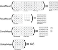
- Mei-Po Kwan (born 1962) - geographer that coined the Uncertain geographic context problem and the neighborhood effect averaging problem.
- Michael DeMers (born 1951) – geographer who wrote numerous books contributing to geographic information systems
- Mark Monmonier (born 1943) – cartographic theorist who wrote numerous books contributing to geographic information systems
- Michael Frank Goodchild (born 1944) – GIS scholar and winner of the RGS founder's medal in 2003
- Richard J. Chorley (1927–2002) - played an instrumental role in bringing in the use of systems theory to geography.[31]
- Roger Tomlinson (1933–2014) – the primary originator of modern geographic information systems
- Stan Openshaw (1946 – 2022) – influential British geographer in the use of computer-based/computational geography
- Kelvyn Jones (born 1953) - developed multilevel models that analyze at multiple scales simultaneously
- Torsten Hägerstrand (1916–2004)- established the discipline of time geography
- Waldo Tobler (1930–2018) – coined the first and second law of geography
- William Bunge (1928–2013) - early quantitative geographer
- William Garrison (1924–2015) - Early leader of the quantitative revolution and one of the founders of regional science.
See also
[edit]- Areography (geography of Mars)
- Concepts and Techniques in Modern Geography
- Design of experiments
- Map communication model
- Modifiable areal unit problem
- Modifiable temporal unit problem
- Neogeography
- Planetary science
- Quantitative history
- Scientific Geography Series
- Uncertain geographic context problem
Notes
[edit]- ^ During the 1940s–1970s, it was customary to capitalize generalized concept names, especially in philosophy ("Truth, Kindness, Beauty"), plus using capital letters when naming ideologies, movements, or schools of thought. Example: "the Automobile" as a concept, versus "the automobile in a garage"
References
[edit]- ^ a b c d e f Fotheringham, A. Stewart; Brunsdon, Chris; Charlton, Martin (2000). Quantitative Geography: Perspectives on Spatial Data Analysis. Sage Publications Ltd. ISBN 978-0-7619-5948-9.
- ^ Murakami, Daisuke; Yamagata, Yoshiki (2020). "Chapter Six - Models in quantitative geography". Spatial Analysis Using Big Data: Methods and Urban Applications. pp. 159–178. doi:10.1016/B978-0-12-813127-5.00006-0. ISBN 9780128131275. S2CID 213700891. Retrieved 3 February 2023.
- ^ a b c Yano, Keiji (2001). "GIS and quantitative geography". GeoJournal. 52 (3): 173–180. doi:10.1023/A:1014252827646. S2CID 126943446.
- ^ Taylor, Peter J. (1977). Quantitative Methods in Geography: An introduction to Spatial Analysis. Prospect Heights, Illinois: Waveland Press, inc. ISBN 0-88133-072-8.
- ^ DeLyser, Dydia; Herbert, Steve; Aitken, Stuart; Crang, Mike; McDowell, Linda (November 2009). The SAGE Handbook of Qualitative Geography (1 ed.). SAGE Publications. ISBN 9781412919913. Retrieved 27 April 2023.
- ^ a b c Murray, Alan T. (February 2010). "Quantitative Geography". Journal of Regional Science. 50 (1): 143–163. Bibcode:2010JRegS..50..143M. doi:10.1111/j.1467-9787.2009.00642.x. S2CID 127919804. Retrieved 3 February 2023.
- ^ Li, Xin; Zheng, Donghai; Feng, Min; Chen, Fahu (November 2021). "Information geography: The information revolution reshapes geography". Science China Earth Sciences. 65 (2): 379–382. doi:10.1007/s11430-021-9857-5.
- ^ Franklin, Rachel (2022). "Quantitative methods I: Reckoning with uncertainty". Progress in Human Geography. 46 (2): 689–697. doi:10.1177/03091325211063635. S2CID 246032475.
- ^ Franklin, Rachel (February 2023). "Quantitative methods II: Big theory". Progress in Human Geography. 47 (1): 178–186. doi:10.1177/03091325221137334. S2CID 255118819.
- ^ Diriwächter, R. & Valsiner, J. (January 2006) Qualitative Developmental Research Methods in Their Historical and Epistemological Contexts. FQS. Vol 7, No. 1, Art. 8
- ^ Haggett, Peter (16 July 2008). "The Local Shape of Revolution: Reflections on Quantitative Geography at Cambridge in the 1950s and 1960s". Geographical Analysis. 40 (3): 336–352. Bibcode:2008GeoAn..40..336H. doi:10.1111/j.1538-4632.2008.00731.x. Retrieved 3 February 2023.
- ^ a b Ferreira, Daniela; Vale, Mário (5 Oct 2020). "Geography in the Big Data Age: An Overview of the Historical Resonance of Current Debates". Geographical Review. 112 (2): 250–266. doi:10.1080/00167428.2020.1832424. hdl:10451/44565. S2CID 225166250. Retrieved 3 February 2023.
- ^ a b Tobler, Waldo (1959). "Automation and Cartography". Geographical Review. 49 (4): 526–534. Bibcode:1959GeoRv..49..526T. doi:10.2307/212211. JSTOR 212211. Retrieved 10 March 2022.
- ^ "The 50th Anniversary of GIS". ESRI. Retrieved 18 April 2013.
- ^ Hegarty, Christopher J.; Chatre, Eric (December 2008). "Evolution of the Global Navigation satellite system (GNSS)". Proceedings of the IEEE. 96 (12): 1902–1917. doi:10.1109/JPROC.2008.2006090. S2CID 838848.
- ^ Jensen, John (2016). Introductory digital image processing: a remote sensing perspective. Glenview, IL: Pearson Education, Inc. p. 623. ISBN 978-0-13-405816-0.
- ^ Webber, M J (1980). "Literature for teaching quantitative geography: technique by, for, but not of geographers". Environment and Planning A. 12 (9): 1083–1090. Bibcode:1980EnPlA..12.1083W. doi:10.1068/a121083.
- ^ Hall, Tim (2019). "Reflecting on resources". Journal of Geography in Higher Education. 43 (1): 1–6. doi:10.1080/03098265.2019.1570091.
- ^ Martinez-Galarraga, Julio; Silvestre, Javier; Tirado-Fabregat, Daniel A. (24 August 2023). "Quantitative Economic Geography and Economic History". In Diebolt, Claude; Haupert, Michael (eds.). Handbook of Cliometrics. Berlin, Heidelberg: Springer. doi:10.1007/978-3-642-40458-0_119-1. ISBN 978-3-642-40458-0. Retrieved 15 December 2023.
- ^ DeLyser, Dydia; Herbert, Steve; Aitken, Stuart; Crang, Mike; McDowell, Linda (November 2009). The SAGE Handbook of Qualitative Geography (1 ed.). SAGE Publications. ISBN 9781412919913. Retrieved 27 April 2023.
- ^ Yano, Keiji (2001). "GIS and quantitative geography". GeoJournal. 52 (3): 173–180. doi:10.1023/A:1014252827646. S2CID 126943446.
- ^ "The 'Quantitative Revolution': hard science or "inconsequential claptrap"?". University of Aberdeen. GG3012(NS) Lecture 4. 2011. Archived from the original on 24 February 2015. Retrieved 4 February 2023.
- ^ Gregory, Derek; Johnston, Ron; Pratt, Geraldine; Watts, Michael J.; Whatmore, Sarah (2009). The Dictionary of Human Geography (5th ed.). US & UK: Wiley-Blackwell. pp. 611–12.
- ^ Walker, Robert Toovey (28 Apr 2021). "Geography, Von Thünen, and Tobler's first law: Tracing the evolution of a concept". Geographical Review. 112 (4): 591–607. doi:10.1080/00167428.2021.1906670. S2CID 233620037.
- ^ a b Haidu, Ionel (2016). "What is Technical Geography – a letter from the editor". Geographia Technica. 11: 1–5. doi:10.21163/GT_2016.111.01.
- ^ a b c Goodchild, Michael (2004). "The Validity and Usefulness of Laws in Geographic Information Science and Geography". Annals of the Association of American Geographers. 94 (2): 300–303. doi:10.1111/j.1467-8306.2004.09402008.x. S2CID 17912938.
- ^ a b c Tobler, Waldo (2004). "On the First Law of Geography: A Reply". Annals of the Association of American Geographers. 94 (2): 304–310. doi:10.1111/j.1467-8306.2004.09402009.x. S2CID 33201684. Retrieved 10 March 2022.
- ^ Arbia, Giuseppe; Benedetti, R.; Espa, G. (1996). ""Effects of MAUP on image classification"". Journal of Geographical Systems. 3: 123–141.
- ^ Smith, Peter (2005). "The laws of geography". Teaching Geography. 30 (3): 150.
- ^ Fotheringham, A. Stewart (2006). "Quantification, Evidence and Positivism". In Aitken, Stuart; Valentine, Gil (eds.). Approaches to Human Geography. Sage.
- ^ Jackson, Michael C (2000). Systems approaches to management. Springer Science & Business Media. doi:10.1007/b100327. ISBN 0-306-46500-0.
| |||||||||
| Branches |
| ||||||||
| Techniques and tools |
| ||||||||
| Institutions, organizations, and societies | |||||||||
| Education | |||||||||
| Publication | |||||||||