Rietveld refinement
Rietveld refinement
Main page

Rietveld refinement

logo
Community Hub0 subscribers
Read side by side
from Wikipedia

Rietveld refinement is a technique described by Hugo Rietveld for use in the characterisation of crystalline materials. The neutron and X-ray diffraction of powder samples results in a pattern characterised by reflections (peaks in intensity) at certain positions. The height, width and position of these reflections can be used to determine many aspects of the material's structure.

The Rietveld method uses a least squares approach to refine a theoretical line profile until it matches the measured profile. The introduction of this technique was a significant step forward in the diffraction analysis of powder samples as, unlike other techniques at that time, it was able to deal reliably with strongly overlapping reflections.

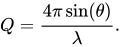
The method was first implemented in 1967,[1] and reported in 1969[2] for the diffraction of monochromatic neutrons where the reflection-position is reported in terms of the Bragg angle, 2θ. This terminology will be used here although the technique is equally applicable to alternative scales such as x-ray energy or neutron time-of-flight. The only wavelength and technique independent scale is in reciprocal space units or momentum transfer Q, which is historically rarely used in powder diffraction but very common in all other diffraction and optics techniques. The relation is
Introduction

[edit]

The most common powder X-ray diffraction (XRD) refinement technique used today is based on the method proposed in the 1960s by Hugo Rietveld.[2] The Rietveld method fits a calculated profile (including all structural and instrumental parameters) to experimental data. It employs the non-linear least squares method, and requires the reasonable initial approximation of many free parameters, including peak shape, unit cell dimensions and coordinates of all atoms in the crystal structure. Other parameters can be guessed while still being reasonably refined. In this way one can refine the crystal structure of a powder material from PXRD data. The successful outcome of the refinement is directly related to the quality of the data, the quality of the model (including initial approximations), and the experience of the user.

The Rietveld method is an incredibly powerful technique which began a remarkable era for powder XRD and materials science in general. Powder XRD is at heart a very basic experimental technique with diverse applications and experimental options. Despite being slightly limited by the one-dimensionality of PXRD data and limited resolution, powder XRD's power is astonishing. It is possible to determine the accuracy of a crystal structure model by fitting a profile to a 1D plot of observed intensity vs angle. Rietveld refinement requires a crystal structure model, and offers no way to come up with such a model on its own. However, it can be used to find structural details missing from a partial or complete ab initio structure solution, such as unit cell dimensions, phase quantities, crystallite sizes/shapes, atomic coordinates/bond lengths, micro strain in crystal lattice, texture, and vacancies.[3][4]

Powder diffraction profiles: peak positions and shapes

[edit]

Before exploring Rietveld refinement, it is necessary to establish a greater understanding of powder diffraction data and what information is encoded therein in order to establish a notion of how to create a model of a diffraction pattern, which is of course necessary in Rietveld refinement. A typical diffraction pattern can be described by the positions, shapes, and intensities of multiple Bragg reflections. Each of the three mentioned properties encodes some information relating to the crystal structure, the properties of the sample, and the properties of the instrumentation. Some of these contributions are shown in Table 1, below.

Powder diffraction pattern as a function of various crystal structure, specimen, and instrumental parameters[5]
Pattern component Crystal structure Specimen property Instrumental parameter
Peak position Unit cell parameters

(a, b, c, α, β, γ)

  • Absorption
  • Porosity
  • Radiation (wavelength),
  • Instrument/sample alignment
  • Axial divergence of the beam
Peak intensity Atomic parameters

(x, y, z, B, etc.)

  • Preferred orientation
  • Absorption
  • Porosity
  • Geometry and configuration
  • Radiation (Lorentz polarization)
Peak shape
  • Crystallinity
  • Disorder
  • Defects
  • Grain size
  • Strain
  • Stress
  • Radiation (spectral purity)
  • Geometry
  • Beam Conditioning

The structure of a powder pattern is essentially defined by instrumental parameters and two crystallographic parameters: unit cell dimensions, and atomic content and coordination. So, a powder pattern model can be constructed as follows:

  1. Establish peak positions: Bragg peak positions are established from Bragg's law using the wavelength and d-spacing for a given unit cell.
  2. Determine peak intensity: Intensity depends on the structure factor, and can be calculated from the structural model for individual peaks. This requires knowledge of the specific atomic coordination in the unit cell and geometrical parameters.
  3. Peak shape for individual Bragg peaks: Represented by functions of the FWHM (which vary with Bragg angle) called the peak shape functions. Realistically ab initio modelling is difficult, and so empirically selected peak shape functions and parameters are used for modelling.
  4. Sum: The individual peak shape functions are summed and added to a background function, leaving behind the resultant powder pattern.

It is easy to model a powder pattern given the crystal structure of a material. The opposite, determining the crystal structure from a powder pattern, is much more complicated. A brief explanation of the process follows, though it is not the focus of this article.

To determine structure from a powder diffraction pattern the following steps should be taken. First, Bragg peak positions and intensities should be found by fitting to a peak shape function including background. Next, peak positions should be indexed and used to determine unit cell parameters, symmetry, and content. Third, peak intensities determine space group symmetry and atomic coordination. Finally, the model is used to refine all crystallographic and peak shape function parameters. To do this successfully, there is a requirement for excellent data which means good resolution, low background, and a large angular range.

Peak shape functions

[edit]

For general application of the Rietveld method, irrespective of the software used, the observed Bragg peaks in a powder diffraction pattern are best described by the so-called peak shape function (PSF). The PSF is a convolution of three functions: the instrumental broadening , wavelength dispersion , and the specimen function , with the addition of a background function, . It is represented as follows:

,

where denotes convolution, which is defined for two functions and as an integral:

The instrumental function depends on the location and geometry of the source, monochromator, and sample. Wavelength function accounts for the distribution of the wavelengths in the source, and varies with the nature of the source and monochromatizing technique. The specimen function depends on several things. First is dynamic scattering, and secondly the physical properties of the sample such as crystallite size, and microstrain.

A short aside: unlike the other contributions, those from the specimen function can be interesting in materials characterization. As such, average crystallite size, , and microstrain, , effects on Bragg peak broadening, (in radians), can be described as follows, where is a constant:

and .

Returning to the peak shape function, the goal is to correctly model the Bragg peaks which exist in the observed powder diffraction data. In the most general form, the intensity, , of the point (, where is the number of measured points) is the sum of the contributions from the overlapped Bragg peaks (), and the background, , and can be described as follows:

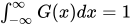
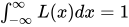
where is the intensity of the Bragg peak, and . Since is a multiplier, it is possible to analyze the behaviour of different normalized peak functions independently of peak intensity, under the condition that the integral over infinity of the PSF is unity. There are various functions that can be chosen to do this with varying degrees of complexity. The most basic functions used in this way to represent Bragg reflections are the Gauss, and Lorentzian functions. Most commonly though, is the pseudo-Voigt function, a weighted sum of the former two (the full Voigt profile is a convolution of the two, but is computationally more demanding). The pseudo-Voigt profile is the most common and is the basis for most other PSF's. The pseudo-Voigt function can be represented as:

,

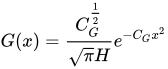
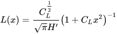
where

and

are the Gaussian and Lorentzian contributions, respectively.

Thus,

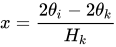
where:

  • and are the full widths at half maximum (FWHM)
  • is essentially the Bragg angle of the point in the powder pattern with its origin in the position of the peak divided by the peak's FWHM.
  • , and and are normalization factors such that and respectively.
  • , known as the Caglioti formula,[6] is the FWHM as a function of for Gauss, and pseudo-Voigt profiles. , , and are free parameters.
  • is the FWHM vs. for the Lorentz function. and are free variables
  • , where is the pseudo-Voigt mixing parameter, and are free variables.

The pseudo-Voigt function, like the Gaussian and Lorentz functions, is a centrosymmetric function, and as such does not model asymmetry. This can be problematic for non-ideal powder XRD data, such as those collected at synchrotron radiation sources, which generally exhibit asymmetry due to the use of multiple focusing optics.

The Finger–Cox–Jephcoat function is similar to the pseudo-Voigt, but has better handling of asymmetry, which is treated in terms of axial divergence. The function is a convolution of pseudo-Voigt with the intersection of the diffraction cone and a finite receiving slit length using two geometrical parameters, , and , where and are the sample and the detector slit dimensions in the direction parallel to the goniometer axis, and is the goniometer radius.[7]

Peak shape as described in Rietveld's paper

[edit]

The shape of a powder diffraction reflection is influenced by the characteristics of the beam, the experimental arrangement, and the sample size and shape. In the case of monochromatic neutron sources the convolution of the various effects has been found to result in a reflex almost exactly Gaussian in shape. If this distribution is assumed then the contribution of a given reflection to the profile at position is:

where is the full width at half peak height (full-width half-maximum), is the center of the reflex, and is the calculated intensity of the reflex (determined from the structure factor, the Lorentz factor, and multiplicity of the reflection).

At very low diffraction angles the reflections may acquire an asymmetry due to the vertical divergence of the beam. Rietveld used a semi-empirical correction factor, to account for this asymmetry:

where is the asymmetry factor and is , , or depending on the difference being positive, zero, or negative respectively.

At a given position more than one diffraction peak may contribute to the profile. The intensity is simply the sum of all reflections contributing at the point .

Integrated intensity

[edit]

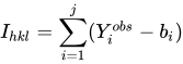
For a Bragg peak , the observed integrated intensity, , as determined from numerical integration is

,

where is the total number of data points in the range of the Bragg peak. The integrated intensity depends on multiple factors, and can be expressed as the following product:


where:

  • : scale factor
  • : multiplicity factor, which accounts for symmetrically equivalent points in the reciprocal lattice
  • : Lorentz multiplier, defined by diffraction geometry
  • : polarization factor
  • : absorption multiplier
  • : preferred orientation factor
  • : extinction factor (often neglected as it is usually insignificant in powders)
  • : structure factor as determined by the crystal structure of the material

Peak width as described in Rietveld's paper

[edit]

The width of the diffraction peaks are found to broaden at higher Bragg angles. This angular dependency was originally represented by

where , , and are the half-width parameters and may be refined during the fit.

Preferred orientation

[edit]

In powder samples there is a tendency for plate- or rod-like crystallites to align themselves along the axis of a cylindrical sample holder. In solid polycrystalline samples the production of the material may result in greater volume fraction of certain crystal orientations (commonly referred to as texture). In such cases the reflex intensities will vary from that predicted for a completely random distribution. Rietveld allowed for moderate cases of the former by introducing a correction factor:

where is the intensity expected for a random sample, is the preferred orientation parameter and is the acute angle between the scattering vector and the normal of the crystallites.

Refinement

[edit]

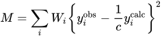
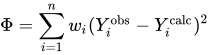
The principle of the Rietveld method is to minimize a function which analyzes the difference between a calculated profile and the observed data . Rietveld defined such an equation as:

where is the statistical weight and is an overall scale factor such that .

Least squares method

[edit]

The fitting method used in Rietveld refinement is the non-linear least squares approach. A detailed derivation of non-linear least squares fitting will not be given here. Further detail can be found in Chapter 6 of Pecharsky and Zavalij's text 12 . There are a few things to note however. First, non-linear least squares fitting has an iterative nature for which convergence may be difficult to achieve if the initial approximation is too far from correct, or when the minimized function is poorly defined. The latter occurs when correlated parameters are being refined at the same time, which may result in divergence and instability of the minimization. This iterative nature also means that convergence to a solution does not occur immediately for the method is not exact. Each iteration depends on the results of the last which dictate the new set of parameters used for refinement. Thus, multiple refinement iterations are required to eventually converge to a possible solution.

Rietveld method basics

[edit]

Using non-linear least squares minimization, the following system is solved:
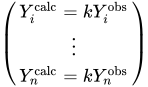
where is the calculated intensity and is the observed intensity of a point in the powder pattern, , is a scale factor, and is the number of measured data points. The minimized function is given by:

where is the weight, and from the previous equation is unity (since is usually absorbed in the phase scale factor). The summation extends to all data points. Considering the peak shape functions and accounting for the overlapping of Bragg peaks because of the one-dimensionality of XRD data, the expanded form of the above equation for the case of a single phase measured with a single wavelength becomes:


where:

  • is the background at the data point.
  • is the phase scale factor.
  • is the number of Bragg reflections contributing to the intensity of the reflection.
  • is the integrated intensity of the Bragg peak.
  • is the peak shape function.

For a material that contains several phases (), the contribution from each is accounted for by modifying the above equation as follows:


It can easily be seen from the above equations that experimentally minimizing the background, which holds no useful structural information, is paramount for a successful profile fitting. For a low background, the functions are defined by contributions from the integrated intensities and peak shape parameters. But with a high background, the function being minimized depends on the adequacy of the background and not integrated intensities or peak shapes. Thus, a structure refinement cannot adequately yield structural information in the presence of a large background.

It is also worth noting the increased complexity brought forth by the presence of multiple phases. Each additional phase adds to the fitting, more Bragg peaks, and another scale factor tied to corresponding structural parameters, and peak shape. Mathematically they are easily accounted for, but practically, due to the finite accuracy and limited resolution of experimental data, each new phase can lower the quality and stability of the refinement. It is advantageous to use single phase materials when interested in finding precise structural parameters of a material. However, since the scale factors of each phase are determined independently, Rietveld refinement of multi phase materials can quantitatively examine the mixing ratio of each phase in the material.

Refinement parameters

[edit]

Background

[edit]

Generally, the background is calculated as a Chebyshev polynomial. In GSAS and GSAS-II they appear as follows. Again, background is treated as a Chebyshev polynomial of the first kind ("Handbook of Mathematical Functions", M. Abramowitz and IA. Stegun, Ch. 22), with intensity given by:
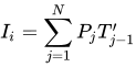
where are the coefficients of the Chebyshev polynomial taken from Table 22.3, pg. 795 of the Handbook. The coefficients have the form:

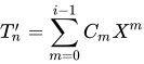
and the values for are found in the Handbook. The angular range () is converted to to make the Chebyshev polynomial orthogonal by

And, the orthogonal range for this function is –1 to +1.

Sample displacement: sample transparency and zero-shift corrections

Different correction factors have been developed to account for the specimen-detector displacement in Debye-Scherrer [8] (transmission) and Bragg-Brentano[9] (reflection) geometries. Correction factors have been published for flat tilted and non-tilted 2D detectors as well.[10][11]

Traditional X-ray diffraction experiments place the detector normal to the incident X-ray beam, centering the detector on the beam or placing the incident beam at the bottom edge of the detector. In these experiments, a unique configuration is taken by aligning the detector such that the incident X-rays are still hitting the bottom-most edge of the detector. However, tilting the detector forward such that the topmost edge of it is directly above the sample provides a number of benefits such as higher quality and better resolved radial distribution functions than in typical traditional geometries, improved dynamic range, increased reciprocal space resolution per pixel for low angle scattering and access to higher reciprocal space values at lower energies.[12] Tilting the detector does not have much impact when carrying out SAXS experiments, however it has a huge impact on WAXS measurements in large-scale facilities (synchrotrons).

Sample-detector displacement correction with flat 2D detectors and non-conventional geometries

The appropriate function for the correction of peak positions due to sample displacement depends upon the geometry of the instrument. Guzmán’s equation[11] provides the correction with flat detectors generalized to non-conventional geometries in both reflection and transmission modes:

where corresponds to the tilt (angle) of the detector, and are the corrected and uncorrected values of the diffraction angles, respectively, is the uncorrected sample-to-detector distance, is the correction for the sample-to-detector distance (corrected sample-to-detector distance ).

Other parameters

[edit]

Now, given the considerations of background, peak shape functions, integrated intensity, and non-linear least squares minimization, the parameters used in the Rietveld refinement which put these things together can be introduced. Below are the groups of independent least squares parameters generally refined in a Rietveld refinement.

  • Background parameters: usually 1 to 12 parameters.
  • Sample displacement: sample transparency, and zero shift corrections. (move peak position)
  • Multiple peak shape parameters.
    • FWHM parameters: i.e. Caglioti parameters (see section 3.1.2)
    • Asymmetry parameters (FCJ parameters)
  • Unit cell dimensions
    • one to six parameters (a, b, c, α, β, γ), depending on the crystal family/system, for each present phase.
  • Preferred orientation, and sometimes absorption, porosity, and extinction coefficients, which can be independent for each phase.
  • Scale factors (for each phase)
  • Positional parameters of all independent atoms in the crystal model (generally 0 to 3 per atom).
  • Population parameters
    • Occupation of site positions by atoms.
  • Atomic displacement parameters
    • Isotropic and anisotropic (temperature) parameters.

Each Rietveld refinement is unique and there is no prescribed sequence of parameters to include in a refinement. It is up to the user to determine and find the best sequence of parameters for refinement. It is worth noting that it is rarely possible to refine all relevant variables simultaneously from the beginning of a refinement, nor near the end since the least squares fitting will be destabilized or lead to a false minimum. It is important for the user to determine a stopping point for a given refinement. Given the complexity of Rietveld refinement it is important to have a clear grasp of the system being studied (sample, and instrumentation) to ensure that results are accurate, realistic, and meaningful. High data quality, a large enough range, and a good model – to serve as the initial approximation in the least squares fitting – are necessary for a successful, reliable, and meaningful Rietveld refinement.

Figures of merit

[edit]

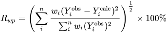
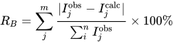
Since refinement depends on finding the best fit between a calculated and experimental pattern, it is important to have a numerical figure of merit quantifying the quality of the fit. Below are the figures of merit generally used to characterize the quality of a refinement. They provide insight to how well the model fits the observed data.

Profile residual (reliability factor):
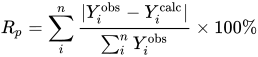
Weighted profile residual:
Bragg residual:
Expected profile residual:
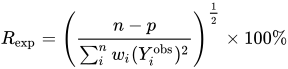
Goodness of fit:

It is worth mentioning that all but one () figure of merit include a contribution from the background. There are some concerns about the reliability of these figures, as well there is no threshold or accepted value which dictates what represents a good fit.[13] The most popular and conventional figure of merit used is the goodness of fit which should approach unity given a perfect fit, though this is rarely the case. In practice, the best way to assess quality is a visual analysis of the fit by plotting the difference between the observed and calculated data plotted on the same scale.

References

[edit]

Notes

[edit]
Revisions and contributorsEdit on WikipediaRead on Wikipedia
from Grokipedia
Rietveld refinement is a least-squares method for refining crystal structures from powder diffraction data, where a calculated diffraction profile, based on a structural model, is fitted to the entire observed pattern to determine parameters such as atomic positions, site occupancies, lattice constants, and thermal displacements.[1] Developed by Dutch physicist Hugo M. Rietveld in 1969 while working at the Reactor Centrum Nederland, the technique was initially applied to neutron powder diffraction for nuclear and magnetic structure analysis but quickly extended to X-ray and synchrotron data.[2] By modeling overlapping peaks and background contributions through analytical profile functions—such as Gaussian, Lorentzian, or pseudo-Voigt—the method overcomes limitations of traditional single-peak intensity extraction, enabling precise structural characterization even from polycrystalline samples. The Rietveld method revolutionized powder crystallography by providing a full-pattern fitting approach that incorporates instrumental resolution, sample microstructure (e.g., crystallite size and microstrain broadening), and preferred orientation effects, resulting in more reliable quantitative phase analysis and structural refinements. Key to its success is the iterative refinement process, which minimizes the weighted difference between observed and calculated intensities using figures of merit like the weighted profile R-factor (R_wp) and goodness-of-fit (χ²), with convergence typically assessed when parameter shifts are less than 0.1 times their estimated standard deviations. Originally implemented in Fortran code for mainframe computers, modern software packages like GSAS, FullProf, and TOPAS facilitate its use across diverse applications, from materials science to pharmaceutical development.[2] Over the past five decades, Rietveld refinement has become the standard for analyzing complex multiphase materials, with its original 1969 publication cited more than 22,000 times as of 2025, underscoring its foundational role in advancing structural science.[3] Guidelines from the International Union of Crystallography emphasize high-quality data collection—such as step sizes such that there are approximately 5–10 steps across the width of each peak (or about 10–20% of the full width at half maximum) and sample preparation to minimize absorption and particle size effects (ideally 1–5 µm)—to ensure accurate results.[4] Despite challenges like correlated parameters or amorphous content, restraints on bond lengths and angles, derived from known chemistry, enhance reliability in underdetermined cases.

History and Overview

Development and Origins

The Rietveld method, building on earlier profile refinement work by colleagues Bert O. Loopstra and Bob van Laar, was developed by Hugo M. Rietveld starting around 1965 at the Reactor Centre Netherlands in Petten, Netherlands, where he worked in the neutron diffraction group following his PhD.[5] Initially created to analyze neutron powder diffraction data, the approach addressed key challenges in extracting accurate structural parameters from patterns featuring overlapping reflections, which traditional methods struggled to resolve. This development marked an evolution from conventional single-peak fitting techniques, which relied on isolating and integrating individual Bragg peaks, to a full-profile refinement strategy that modeled the entire diffraction pattern holistically. The motivation stemmed from the inherent limitations of powder data analysis, such as peak overlap and low signal-to-noise ratios in neutron experiments, prompting Rietveld to leverage computational capabilities available at the time, including the Electrologica X8 computer.[5] The foundational description of peak line profiles appeared in a 1967 note in Acta Crystallographica, but the first full implementation of the profile refinement method was detailed in Rietveld's 1969 publication in the Journal of Applied Crystallography.[1] In this seminal work, the method was presented as a least-squares procedure using step-scanned profile intensities rather than integrated intensities. Early applications focused on simple crystalline structures, including the refinement of nuclear parameters in alkaline-earth metal uranates such as Sr₂UO₅.[6] These initial tests highlighted the method's potential to improve precision in structure determination beyond what was achievable with prior techniques.[5]

Basic Principles

Rietveld refinement is a full-pattern fitting technique that employs a least-squares approach to minimize the difference between an observed powder diffraction profile and a calculated profile generated from a structural model.[1] This method directly utilizes the step-scanned intensities of the diffraction pattern, rather than relying on extracted integrated intensities from individual peaks, enabling the refinement of complex structures where overlaps are common.[1] Developed initially for neutron diffraction data on nuclear and magnetic structures, it has since been extended to X-ray powder diffraction, providing a robust framework for quantitative phase analysis and structural determination.[2] The primary goal of Rietveld refinement is to simultaneously optimize structural parameters—such as lattice constants, atomic positions, and site occupancies—along with instrumental factors like peak shape and width parameters, and sample-related effects including background scattering and preferred orientation.[2] By modeling the entire diffraction pattern, the technique extracts more reliable information from the data than methods limited to isolated reflections, particularly in cases of low-resolution or highly overlapping peaks typical of powder samples.[1] This holistic fitting process enhances the accuracy of refined parameters, making it indispensable for materials characterization in fields like crystallography and materials science.[2] The workflow begins with an initial structural model, often derived from single-crystal data or ab initio predictions, which is used to compute the theoretical diffraction profile based on the crystal's space group, atomic coordinates, and scattering factors.[1] This calculated profile is then compared to the experimental data, and parameters are iteratively adjusted via least-squares minimization until the residual difference converges to a minimum, typically assessed by metrics like the profile R-factor.[2] Constraints, such as those ensuring physical plausibility (e.g., bond lengths), may be applied to guide the refinement and prevent divergence.[1] In contrast to single-reflection methods, such as profile-independent analysis that decomposes peaks to obtain individual intensities before refinement, Rietveld refinement leverages the full pattern to inherently account for overlaps and correlations between reflections, improving precision without requiring peak isolation.[2] This distinction addresses the inherent limitations of powder diffraction data, where many reflections contribute to the observed profile, allowing for more comprehensive structural insights.[1]

Powder Diffraction Fundamentals

Peak Positions and Shapes

In powder diffraction patterns, the positions of Bragg peaks are fundamentally determined by Bragg's law, expressed as $ n\lambda = 2d_{hkl} \sin\theta $, where $ n $ is a positive integer representing the diffraction order, $ \lambda $ is the wavelength of the incident radiation, $ d_{hkl} $ is the interplanar spacing for the set of lattice planes with Miller indices $ (hkl) $, and $ \theta $ is the Bragg diffraction angle. The interplanar spacing $ d_{hkl} $ is directly related to the unit cell parameters of the crystal structure through geometric relations specific to the crystal system, such as $ \frac{1}{d_{hkl}^2} = \frac{h^2}{a^2} + \frac{k^2}{b^2} + \frac{l^2}{c^2} $ for an orthorhombic lattice. In Rietveld refinement, these theoretical peak positions are computed from an initial structural model and serve as the foundation for fitting the entire diffraction profile, enabling the refinement of lattice parameters to match observed data.[7][1] Diffraction peak shapes in powder patterns deviate from ideal symmetry due to both instrumental and sample-related effects. Instrumental asymmetry often arises from the use of flat-plate samples in Bragg-Brentano geometry, where the sample surface is not perfectly aligned with the diffractometer circle, leading to defocusing and angular shifts that elongate peaks toward lower $ 2\theta $ angles, particularly for low-angle reflections. Physical contributions to peak shape include broadening from finite crystallite sizes, which produces Lorentzian-like tails due to the limited number of coherently scattering domains, and microstrain from lattice distortions, which adds Gaussian broadening through variations in interplanar spacings. These factors collectively result in asymmetric profiles that must be accurately parameterized for reliable structural analysis in Rietveld methods.[7] Peak shapes are modeled using analytical profile functions to capture both symmetric broadening and asymmetry. A widely adopted function is the pseudo-Voigt profile, defined as
I(2θ)=ηL(2θ;ΓL)+(1η)G(2θ;ΓG), I(2\theta) = \eta \, L(2\theta; \Gamma_L) + (1 - \eta) \, G(2\theta; \Gamma_G),
where $ L $ and $ G $ represent the Lorentzian and Gaussian components, respectively, $ \Gamma_L $ and $ \Gamma_G $ are their respective full widths at half maximum, and $ \eta $ (ranging from 0 to 1) is a refinable mixing parameter that adjusts the relative contributions, often varying with $ 2\theta $ to account for evolving asymmetry. This function approximates the true Voigt convolution while being computationally efficient for whole-pattern fitting. In the seminal work introducing the Rietveld method, peak profiles were modeled using a Gaussian function.[1][8]

Integrated Intensities and Widths

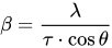
In powder diffraction, the integrated intensity of a Bragg reflection represents the total area under the diffraction peak and serves as a key observable for structural analysis. This intensity IhklI_{hkl} is proportional to the square of the magnitude of the structure factor, Fhkl2|F_{hkl}|^2, which encodes information about atomic positions, site occupancies, and thermal displacements within the crystal lattice. Additionally, IhklI_{hkl} incorporates geometric and experimental factors, including the multiplicity mhklm_{hkl} (accounting for equivalent reflections) and the Lorentz-polarization factor LpL_p (arising from the scanning geometry and beam polarization). The full expression is thus IhklmhklLpFhkl2I_{hkl} \propto m_{hkl} L_p |F_{hkl}|^2, enabling the extraction of refined structural parameters during Rietveld refinement by comparing modeled intensities to observed data. Peak widths in diffraction patterns, quantified by the full width at half maximum (FWHM, denoted β\beta), provide insights into microstructural features such as crystallite size and lattice strain. For crystallite size DD, the Scherrer equation relates β\beta to the average domain size via
D=Kλβcosθ, D = \frac{K \lambda}{\beta \cos \theta},
where KK is a shape factor (typically 0.9–1.0), λ\lambda is the X-ray wavelength, and θ\theta is the Bragg angle; narrower peaks indicate larger crystallites. To disentangle size and strain effects, the Williamson-Hall method employs a linear plot of βcosθ\beta \cos \theta versus sinθ\sin \theta:
βcosθ=KλD+4ϵsinθ, \beta \cos \theta = \frac{K \lambda}{D} + 4 \epsilon \sin \theta,
where ϵ\epsilon is the microstrain; the y-intercept yields size information, while the slope reflects strain broadening. These analyses are integrated into Rietveld refinement to quantify microstructural properties alongside structural refinement. Rietveld's original method modeled peak widths using a Gaussian profile to account for overall broadening from instrumental and sample effects. This unified approach avoids isolating individual peaks for width measurement, instead refining width parameters globally across the pattern to simultaneously optimize intensities and shapes. Through such modeling, site occupancies (affecting scattering power per site) and thermal parameters (via the Debye-Waller factor in FhklF_{hkl}) are determined by minimizing discrepancies between calculated and observed integrated intensities, enhancing the accuracy of atomic-scale models.[1]

Core Refinement Techniques

Least Squares Method

The least squares method serves as the foundational optimization algorithm in Rietveld refinement, enabling the adjustment of structural and instrumental parameters to achieve the best fit between observed and calculated powder diffraction profiles. Developed by Hugo Rietveld in his seminal 1969 paper, this technique adapts classical least squares principles to the entire diffraction pattern, allowing for the extraction of detailed structural information from powder data where single-crystal methods are infeasible. At its core, the method minimizes the chi-squared (χ2\chi^2) statistic, which quantifies the discrepancy between experimental and modeled data:
χ2=iwi(yobs,iycalc,i)2, \chi^2 = \sum_i w_i (y_{obs,i} - y_{calc,i})^2,
where yobs,iy_{obs,i} and ycalc,iy_{calc,i} represent the observed and calculated step intensities at the ii-th point across the profile, and the weights wi=1/σi2w_i = 1/\sigma_i^2 are inversely proportional to the variances σi2\sigma_i^2 of the measurements, ensuring higher-precision data points exert greater influence on the fit. This formulation assumes Gaussian errors in the intensity measurements, a common approximation in powder diffraction analysis. The refinement is inherently nonlinear due to the complex dependence of calculated intensities on parameters, necessitating an iterative solution. Parameter updates Δp\Delta \mathbf{p} are obtained by solving the normal equations:
Δp=(ATWA)1ATWΔy, \Delta \mathbf{p} = (A^T W A)^{-1} A^T W \Delta \mathbf{y},
where A\mathbf{A} is the Jacobian matrix containing partial derivatives ycalc,i/pj\partial y_{calc,i}/\partial p_j of the calculated profile with respect to each refinable parameter pjp_j, WW is the diagonal weight matrix, and Δy=yobsycalc\Delta \mathbf{y} = \mathbf{y}_{obs} - \mathbf{y}_{calc}. To enhance numerical stability, especially with ill-conditioned matrices from correlated parameters or noisy data, implementations often employ gradient-based algorithms like the Levenberg-Marquardt method, which blends steepest descent and Gauss-Newton approaches. Convergence is monitored through criteria such as parameter shifts falling below 0.1 times their estimated standard deviations (esds) or the χ2\chi^2 value stabilizing across iterations, preventing overfitting while ensuring a reliable minimum is reached. The final variance-covariance matrix, computed as the inverse of the weighted curvature matrix (ATWA)(A^T W A) scaled by the reduced χ2\chi^2 (i.e., χ2/(NP)\chi^2 / (N - P), with NN observations and PP parameters), yields the esds along its diagonal and quantifies correlations off-diagonal, highlighting potential parameter interdependencies that may require constraints or sequential refinement strategies. Unlike traditional crystallographic least squares refinements, which operate on extracted integrated intensities of discrete Bragg reflections and thus discard profile shape information, the Rietveld method leverages the full intensity profile—including overlaps and backgrounds—for a more holistic and statistically robust optimization.

Profile Function Modeling

In the Rietveld refinement method, the theoretical diffraction profile is constructed by summing the contributions from all Bragg reflections across the entire powder diffraction pattern. The calculated intensity at each point 2θi2\theta_i is given by
ycalc(2θi)=hklIhklP(2θi2θhkl)+BG(2θi), y_{calc}(2\theta_i) = \sum_{hkl} I_{hkl} \, P(2\theta_i - 2\theta_{hkl}) + BG(2\theta_i),
where IhklI_{hkl} represents the integrated intensity of the (hkl)(hkl) reflection, PP is the normalized profile function describing the shape of an individual peak, 2θhkl2\theta_{hkl} is the calculated Bragg position, and BG(2θi)BG(2\theta_i) accounts for the background intensity.[1] This approach models the entire observed pattern yobs(2θi)y_{obs}(2\theta_i) without isolating individual peaks, enabling a least-squares fit to refine structural and other parameters simultaneously.[1] Rietveld's original formulation, developed for neutron powder diffraction data, employed analytical profile functions to describe peak shapes, assuming Gaussian profiles determined primarily by instrumental resolution.[9] Peak widths were parameterized using the Caglioti relation, FWHM2=Utan2θ+Vtanθ+W\mathrm{FWHM}^2 = U \tan^2\theta + V \tan\theta + W, where UU, VV, and WW are refinable coefficients capturing angular dependence.[1] Later adaptations incorporated more flexible analytical profile functions, such as the pseudo-Voigt or split-Pearson functions, to model deviations from simple Gaussian or Lorentzian shapes, including asymmetry and sample effects, without requiring explicit separation of overlapping contributions. Modern extensions to profile modeling have shifted toward the fundamental parameters approach (FPA), which physically parameterizes the instrumental resolution function based on optical elements like X-ray source emission profiles, monochromator characteristics, and detector responses, rather than empirically fitting ad hoc parameters. In FPA, the overall peak profile is obtained by convolving the intrinsic sample diffraction (e.g., a delta function at 2θhkl2\theta_{hkl}) with the instrumental function and any sample broadening terms, such as crystallite size or microstrain effects. This method, pioneered for X-ray data, reduces the number of refinable parameters and improves transferability across instruments, enhancing accuracy in quantitative phase analysis and microstructural characterization. The Rietveld approach inherently addresses overlapping peaks by refining all profile parameters globally across the pattern, avoiding the need for decomposition into individual reflections.[1] This simultaneous fitting leverages the structural model to correlate intensities and positions, allowing resolution of severe overlaps that would be intractable in traditional peak-by-peak methods.[10]

Refinement Parameters and Strategies

Structural and Instrumental Parameters

In Rietveld refinement, structural parameters define the crystal lattice and atomic arrangement within the unit cell, enabling the calculation of Bragg peak positions and intensities from the known atomic scattering factors. Lattice parameters, including the cell lengths aa, bb, cc and angles α\alpha, β\beta, γ\gamma, are refined to align calculated peak positions with observed diffraction data, often starting with values from single-crystal studies or indexing results.[1][11] Accurate refinement of these parameters requires high-resolution data and correction for instrumental shifts, as small errors can propagate to significant deviations in derived volumes or densities. Atomic coordinates, typically expressed as fractional positions xx, yy, zz for each atom in the asymmetric unit, are refined to optimize the structure factor contributions to peak intensities, with heavier atoms refined before lighter ones to minimize correlations.[1][11] These parameters account for site occupancies in cases of substitutional disorder, ensuring the model reflects the average structure observed in powder data. Displacement parameters, which describe thermal motion or static disorder, are refined as isotropic values BisoB_{iso} for simpler models or anisotropic tensors UijU_{ij} for more detailed analyses, with neutron diffraction providing superior sensitivity due to scattering from nuclei rather than electrons.[2][11] Refinement proceeds cautiously, often grouping similar atoms to avoid divergence from correlated shifts in coordinates and displacements. Instrumental parameters correct for systematic errors in the diffraction setup, ensuring the calculated profile matches the experimental pattern across the angular range. The zero-point error, representing the angular offset at 2θ = 0°, is refined alongside lattice parameters to adjust peak positions, typically calibrated using a standard like NIST SRM 640b for precision better than 0.01°.[11] Wavelength calibration accounts for any deviation from the nominal value in the incident beam, essential for absolute d-spacing determination. The scale factor normalizes the overall intensity of the calculated pattern to the observed data, while absorption corrections address sample transparency or μρ effects, particularly in transmission geometry for accurate intensity scaling.[2][11] For multi-phase samples, phase-related parameters include weight fractions, calculated as Wα=SαZα[Mα](/page/Molecularmass)VαSiZiMiViW_\alpha = \frac{S_\alpha Z_\alpha [M_\alpha](/page/Molecular_mass) V_\alpha}{\sum S_i Z_i M_i V_i} where SαS_\alpha is the refined scale factor, ZαZ_\alpha the number of formula units, MαM_\alpha the molecular mass, and VαV_\alpha the unit cell volume for phase α\alpha, enabling quantitative analysis without external standards. Unit cell variations across phases are refined independently to capture compositional differences, with the sum of fractions constrained to unity.[2] To maintain physical realism and convergence in refinements with limited data, constraints fix relationships between parameters, such as linking occupancies in solid solutions to maintain charge balance or composition.[11] Restraints, applied as soft penalties, enforce expected bond lengths or angles based on prior chemical knowledge, weighted by an empirical factor to balance geometric and diffraction data without over-constraining the model. These techniques are particularly vital for complex or low-symmetry structures, reducing parameter correlations and improving precision.[2]

Background and Preferred Orientation

In Rietveld refinement, the background scattering component arises from various sources such as air scattering, sample holder contributions, and incoherent processes like Compton scattering or fluorescence, necessitating explicit modeling to isolate the Bragg diffraction signals accurately. Empirical polynomial functions, particularly shifted Chebyshev polynomials of the first kind, are widely employed for this purpose due to their flexibility in fitting smooth, slowly varying backgrounds without introducing unphysical oscillations. The background intensity is typically expressed as $ BG(2\theta) = \sum_{k=1}^{n} c_k T_k(2\theta - \gamma) $, where $ T_k $ are the shifted Chebyshev polynomials, $ c_k $ are refinable coefficients, $ 2\theta $ is the scattering angle, $ \gamma $ is a shift parameter to ensure orthogonality over the data range, and $ n $ is the number of terms selected based on the pattern's complexity to avoid overfitting. For cases involving significant incoherent scattering, physical models incorporating Compton profiles or fluorescence corrections can supplement or replace polynomials, particularly in high-energy X-ray experiments where such contributions are pronounced. Detection of background inadequacies during refinement involves visual inspection of residuals between observed and calculated profiles, where systematic positive or negative deviations in inter-peak regions signal the need for adjustment; strategies typically begin with a fixed low-order polynomial (e.g., 3-6 terms) refined after initial scale and zero-angle parameters, progressing to higher orders or physical terms only if residuals persist. Refinable coefficients $ c_k $ allow adaptation to experimental variations, but fixed constraints on higher-order terms prevent divergence in noisy data, ensuring convergence while maintaining physical realism. These corrections directly influence the scaling of integrated intensities, as unmodeled background inflates or suppresses peak areas, thereby affecting phase quantification and structural reliability. Preferred orientation, or texture, introduces intensity distortions in powder diffraction patterns when crystallites align preferentially due to particle morphology or preparation methods, leading to over- or under-representation of specific $ hkl $ reflections. The March-Dollase model addresses uniaxial textures by applying a correction factor to the structure factor multiplicity, assuming ellipsoidal distribution of orientations around a preferred axis, and is particularly effective for moderate anisotropies where the direction is known a priori from morphology. For more complex, fiber-like or multi-axial textures, spherical harmonics expansions provide a general framework, modeling the orientation distribution function as $ \alpha_{hkl} = \sum_{m=0}^{l_{\max}} g_m Y_m(\gamma) $, where $ Y_m $ are spherical harmonics, $ g_m $ are refinable coefficients up to order $ l_{\max} $ (often 4-8 for convergence), and $ \gamma $ is the angle between the scattering vector and the sample normal. Detection relies on discrepancies in relative peak intensities compared to a random powder standard, with initial indicators from enhanced basal peaks in platy materials or axial reflections in elongated ones. Refinement strategies for preferred orientation commence after profile and lattice parameters are stable, introducing fixed initial values (e.g., March parameter $ G = 1 $ for isotropy) and refining stepwise to avoid correlations with scale factors; higher-order harmonics require symmetry constraints to reduce parameters and ensure stability. In anisotropic materials like clays, where platy habits induce strong (00l) alignment, or fibers exhibiting axial textures, uncorrected preferred orientation can bias site occupancies and thermal parameters by up to 20-50% in affected reflections, underscoring the need for these models to achieve quantitative accuracy in phase analysis and microstructure inference.

Evaluation and Applications

Figures of Merit

In Rietveld refinement, figures of merit provide quantitative assessments of the agreement between the observed powder diffraction pattern and the model calculated from the refined structural parameters, as well as the overall statistical reliability of the fit. These metrics are derived from the least-squares minimization process and are essential for evaluating refinement quality, though they must be interpreted alongside visual inspection of difference plots. The profile R-factor ($ R_p $) measures the unweighted discrepancy between observed and calculated diffraction intensities across the entire profile:
Rp=100(yobsycalc)2yobs2 R_p = 100 \sqrt{ \frac{ \sum (y_{obs} - y_{calc})^2 }{ \sum y_{obs}^2 } }
where $ y_{obs} $ and $ y_{calc} $ represent the observed and calculated step intensities, respectively. A weighted counterpart, the weighted profile R-factor ($ R_{wp} $), incorporates measurement uncertainties via weights $ w_i = 1 / \sigma_i^2 $:
Rwp=100wi(yobs,iycalc,i)2wiyobs,i2 R_{wp} = 100 \sqrt{ \frac{ \sum w_i (y_{obs,i} - y_{calc,i})^2 }{ \sum w_i y_{obs,i}^2 } }
These profile factors quantify how well the entire diffraction pattern, including background and peak shapes, matches the model; $ R_{wp} $ is preferred as it penalizes larger errors more heavily. Typical values for $ R_{wp} $ below 10% indicate a good fit for standard X-ray diffraction data, though this can vary with instrumental resolution and sample quality—lower thresholds (e.g., 2–5%) are common for high-resolution neutron data. The Bragg R-factor ($ R_B $) focuses specifically on the agreement between observed and calculated integrated Bragg intensities, which relate directly to structure factors:
RB=100IobsIcalc2Iobs2 R_B = 100 \sqrt{ \frac{ \sum |I_{obs} - I_{calc}|^2 }{ \sum I_{obs}^2 } }
where $ I_{obs} $ and $ I_{calc} $ are the extracted or modeled integrated intensities for each reflection. This metric is particularly useful for assessing the structural model's accuracy, independent of profile shape details, and values under 5–8% are generally indicative of reliable structure factor refinement. The goodness-of-fit (GoF) evaluates the fit relative to the expected statistical variance and is defined as GoF = R_wp / R_exp, where R_exp = 100 \sqrt{(N - P) / \sum w_i y_{obs,i}^2} is the expected weighted profile R-factor, with $ N $ as the number of data points and $ P $ as the number of refined parameters. An ideal GoF near 1 suggests the model adequately explains the data without overfitting or underfitting; values significantly above 1 may indicate unmodeled systematic errors, while those below 1 could reflect overestimated uncertainties. These figures of merit are sensitive to background modeling, as incorrect background subtraction can inflate $ R_p $ and $ R_{wp} $ by including non-structural contributions in the profile comparison. Additionally, they do not capture preferred orientation or sample-related artifacts, necessitating complementary diagnostics.

Practical Applications and Limitations

Rietveld refinement is widely applied in quantitative phase analysis (QPA) of multiphase mixtures, enabling precise determination of phase fractions without internal standards by scaling structure factors to match observed intensities.[12] This method excels in complex systems where traditional single-peak methods fail due to overlapping reflections, achieving accuracies within ±1-3 wt% for crystalline components in geological and ceramic samples.[13] In microstructure characterization, it models diffraction peak broadening to quantify crystallite size and microstrain, providing insights into defect distributions and anisotropic broadening via integral breadth or Williamson-Hall approaches integrated into the refinement.[14] For instance, refinements of ceria nanoparticles yield crystallite sizes on the order of 15 nm, correlating with synthesis conditions.[15] In-situ studies leverage Rietveld refinement to track dynamic phase transformations in real time, particularly in battery materials under electrochemical cycling. High-energy synchrotron XRD combined with refinement reveals lithium insertion mechanisms in cathodes like Li-rich layered oxides, quantifying evolving phase fractions during charging.[16] Integration with pair distribution function (PDF) analysis extends Rietveld to total scattering data, coupling long-range crystallographic models with local atomic correlations for nanomaterials and disordered systems. This hybrid approach refines both Bragg and diffuse scattering, elucidating short-range order in illite clays or zeolite-encapsulated selenium clusters.[17][18] Practical case studies highlight its utility in pharmaceuticals for polymorph identification and quantification, where form stability affects bioavailability. In famotidine tablets, Rietveld QPA detects trace polymorphic impurities at levels of a few percent, ensuring regulatory compliance without destructive sampling.[19] In materials science, it quantifies fractions in Fe-B-Nb alloys to optimize magnetic properties.[20] Figures of merit like the weighted profile R-factor (R_wp < 10%) validate these analyses, confirming model reliability.[21] Despite its strengths, Rietveld refinement requires an accurate starting structural model; poor initial parameters lead to convergence failures or artifacts in refined occupancies.[22] Amorphous content complicates fits by elevating the background, often necessitating separate modeling or underestimating crystalline phases in nanocomposites.[22] Peak overlap in complex, low-symmetry systems amplifies errors from profile asymmetry, while radiation damage during prolonged synchrotron exposure induces phase changes, degrading data quality.[22] Modern advancements address these challenges through total scattering refinements that unify Rietveld with PDF for comprehensive structural probing, as in high-pressure studies of layered chalcogenides.[23] Post-2020 developments incorporate machine learning to optimize starting models and automate phase quantification, reducing refinement time for large datasets from hours to minutes while improving accuracy in noisy data from various applications.[24]
User Avatar
No comments yet.