Hubbry Logo
Stock and flowStock and flowMain
Open search
Stock and flow
Community hub
Stock and flow
logo
8 pages, 0 posts
0 subscribers
Be the first to start a discussion here.
Stock and flow
Stock and flow
from Wikipedia
Stock vs. flow
Dynamic stock and flow diagram

Economics, business, accounting, and related fields often distinguish between quantities that are stocks and those that are flows. These differ in their units of measurement. A stock is measured at one specific time, and represents a quantity existing at that point in time (say, December 31, 2004), which may have accumulated in the past. A flow variable is measured over an interval of time. Therefore, a flow would be measured per unit of time (say a year). Flow is roughly analogous to rate or speed in this sense.

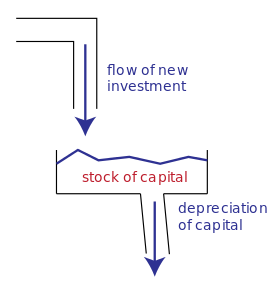
For example, U.S. nominal gross domestic product refers to a total number of dollars spent over a time period, such as a year. Therefore, it is a flow variable, and has units of dollars/year. In contrast, the U.S. nominal capital stock is the total value, in dollars, of equipment, buildings, and other real productive assets in the U.S. economy, and has units of dollars. The diagram provides an intuitive illustration of how the stock of capital currently available is increased by the flow of new investment and depleted by the flow of depreciation.

Stocks and flows in accounting

[edit]

Thus, a stock refers to the value of an asset at a balance date (or point in time), while a flow refers to the total value of transactions (sales or purchases, incomes or expenditures) during an accounting period. If the flow value of an economic activity is divided by the average stock value during an accounting period, we obtain a measure of the number of turnovers (or rotations) of a stock in that accounting period. Some accounting entries are normally always represented as a flow (e.g. profit or income), while others may be represented both as a stock or as a flow (e.g. capital).

A person or country might have stocks of money, financial assets, liabilities, wealth, real means of production, capital, inventories, and human capital (or labor power). Flow magnitudes include income, spending, saving, debt repayment, fixed investment, inventory investment, and labor utilization. These differ in their units of measurement. Capital is a stock concept which yields a periodic income which is a flow concept.

Comparing stocks and flows

[edit]

Stocks and flows have different units and are thus not commensurable – they cannot be meaningfully compared, equated, added, or subtracted. However, one may meaningfully take ratios of stocks and flows, or multiply or divide them. This is a point of some confusion for some economics students, as some confuse taking ratios (valid) with comparing (invalid).

The ratio of a stock over a flow has units of (units)/(units/time) = time. For example, the debt to GDP ratio has units of years (as GDP is measured in, for example, dollars per year whereas debt is measured in dollars), which yields the interpretation of the debt to GDP ratio as "number of years to pay off all debt, assuming all GDP devoted to debt repayment".

The ratio of a flow to a stock has units 1/time. For example, the velocity of money is defined as nominal GDP / nominal money supply; it has units of (dollars / year) / dollars = 1/year.

In discrete time, the change in a stock variable from one point in time to another point in time one time unit later (the first difference of the stock) is equal to the corresponding flow variable per unit of time. For example, if a country's stock of physical capital on January 1, 2010 is 20 machines and on January 1, 2011 is 23 machines, then the flow of net investment during 2010 was 3 machines per year. If it then has 27 machines on January 1, 2012, the flow of net investment during 2010 and 2011 averaged machines per year.

In continuous time, the time derivative of a stock variable is a flow variable.

More general uses

[edit]

Stocks and flows also have natural meanings in many contexts outside of economics, business and related fields. The concepts apply to many conserved quantities such as energy, and to materials such as in stoichiometry, water reservoir management, and greenhouse gases and other durable pollutants that accumulate in the environment or in organisms. Climate change mitigation, for example, is a fairly straightforward stock and flow problem with the primary goal of reducing the stock (the concentration of durable greenhouse gases in the atmosphere) by manipulating the flows (reducing inflows such as greenhouse gas emissions into the atmosphere, and increasing outflows such as carbon dioxide removal). In living systems, such as the human body, energy homeostasis describes the linear relationship between flows (the food we eat and the energy we expend along with the wastes we excrete) and the stock (manifesting as our gain or loss of body weight over time). In Earth system science, many stock and flow problems arise, such as in the carbon cycle, the nitrogen cycle, the water cycle, and Earth's energy budget. Thus stocks and flows are the basic building blocks of system dynamics models. Jay Forrester originally referred to them as "levels" rather than stocks, together with "rates" or "rates of flow".[1]

A stock (or "level variable") in this broader sense is some entity that is accumulated over time by inflows and/or depleted by outflows. Stocks can only be changed via flows. Mathematically a stock can be seen as an accumulation or integration of flows over time – with outflows subtracting from the stock. Stocks typically have a certain value at each moment of time – e.g. the number of population at a certain moment, or the quantity of water in a reservoir.

A flow (or "rate") changes a stock over time. Usually we can clearly distinguish inflows (adding to the stock) and outflows (subtracting from the stock). Flows typically are measured over a certain interval of time – e.g., the number of births over a day or month.

Synonyms

Stock Flow
Level Rate
Integral Derivative
State Variable

Examples

[edit]

Accounting, finance, etc.

[edit]
"Stock" Possible units of stock "Inflow(s)" "Outflow(s)" Possible units of flow
bank balance yen deposits
interest
withdrawals yen per month
inventory of lumber board feet incoming lumber outgoing lumber board feet per week
housing stock dollars

or housing units

housing investment

or new homes built

housing depreciation

or housing units lost

dollars per year

or units of housing

equity shareholdings company shares purchases of shares sales of shares shares per month

Other contexts

[edit]
"Stock" Possible units of stock "Inflow(s)" "Outflow(s)" Possible units of flow
CO2 in atmosphere tons tons emitted tons sequestered tons per day
guests in a hotel persons guests arriving guests leaving persons per day
population persons births
immigration
deaths
emigration
persons per year
water in bathtub liters water pouring in water draining out liters per second
waste in disposal site tons dumping waste decay of waste tons per week
fuel tank gallons refueling fuel consumption gallons per month

Calculus interpretation

[edit]

If the quantity of some stock variable at time is , then the derivative is the flow of changes in the stock. Likewise, the stock at some time is the integral of the flow from some moment set as zero until time .

For example, if the capital stock is increased gradually over time by a flow of gross investment and decreased gradually over time by a flow of depreciation , then the instantaneous rate of change in the capital stock is given by

where the notation refers to the flow of net investment, which is the difference between gross investment and depreciation.

Example of dynamic stock and flow diagram

[edit]
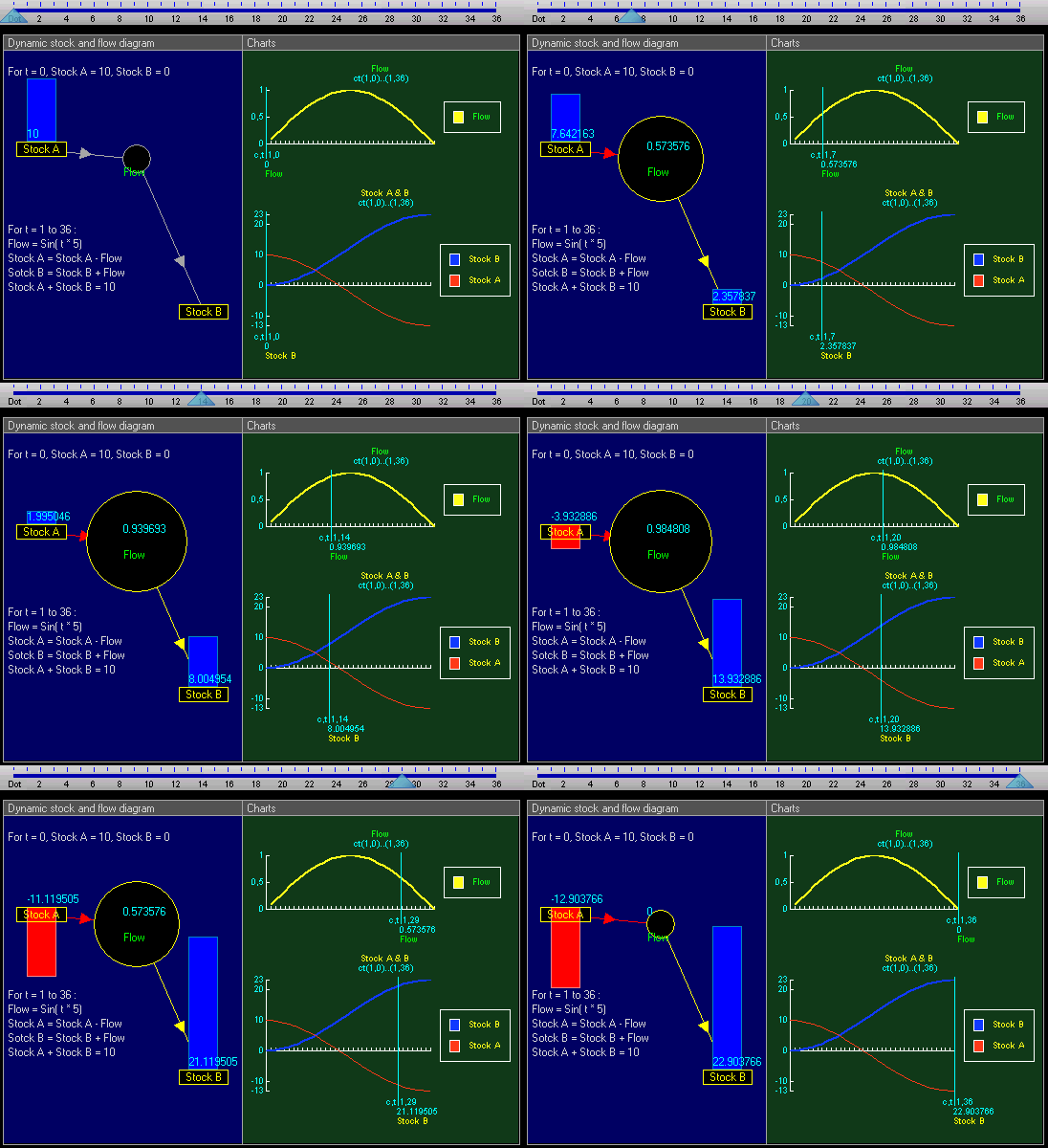
Dynamic stock and flow diagram
Ten first stocks and flow values

Equations that change the two stocks via the flow are:

List of all the equations, in their order of execution in each time, from time = 1 to 36:

History

[edit]

The distinction between a stock and a flow variable is elementary, and dates back centuries in accounting practice (distinction between an asset and income, for instance). In economics, the distinction was formalized and terms were set in (Fisher 1896), in which Irving Fisher formalized capital (as a stock).

Polish economist Michał Kalecki emphasized the centrality of the distinction of stocks and flows, caustically calling economics "the science of confusing stocks with flows" in his critique of the quantity theory of money (circa 1936, frequently quoted by Joan Robinson).[2]

See also

[edit]

References

[edit]
Revisions and contributorsEdit on WikipediaRead on Wikipedia
from Grokipedia
In , , and related disciplines, stocks and flows are fundamental concepts that describe the structure and dynamics of complex by differentiating between accumulated quantities and the rates at which they change. A stock refers to the level or accumulation of a variable measurable at a specific point in time, such as the water in a , the of a , or the in a , acting as a buffer, delay, or of past flows within the . In contrast, a flow is the rate of change affecting a over a defined period, encompassing inflows that increase the (e.g., births or deposits) and outflows that decrease it (e.g., deaths or withdrawals), with the net effect determining whether the rises, falls, or remains in dynamic equilibrium. In , these concepts underpin national , balance sheets, and macroeconomic models, where represent the positions of assets and liabilities at a moment—such as capital , household wealth, or outstanding —valued at market prices or equivalents, while flows denote the economic value created, exchanged, or extinguished over time through transactions like , expenditure, or . The interplay between and flows ensures consistency in economic analysis; for example, changes in financial assets (a ) arise from flows such as acquisitions, disposals, or holding gains, allowing policymakers to track sustainability in areas like fiscal balances or . This framework reveals potential imbalances, such as when outflows exceed inflows, leading to erosion, and is central to stock-flow consistent models that integrate sectoral balance sheets to simulate economy-wide interactions. Beyond , stocks and flows inform systems dynamics modeling for environmental, social, and organizational challenges, emphasizing delays and feedback loops that amplify oscillations or stabilize systems—for instance, in where harvest flows deplete stocks, or in where flows regulate stocks. Their application extends to efforts, revealing leverage points for intervention, such as adjusting flow rates to preserve critical stocks like or .

Core Concepts

Definition of Stocks

In and , a refers to a or variable that measures the amount of a particular entity accumulated at a specific point in time, serving as a snapshot of its magnitude without reference to duration. This static measurement captures the cumulative result of prior processes, distinguishing it from dynamic changes, and is essential for understanding the state of systems at any given instant. Common examples illustrate this concept clearly: the level of water in a bathtub at noon represents the stock of water, independent of how it arrived there; similarly, the population size of a country on a census date or the inventory of goods held by a business at the end of a quarter qualifies as a stock. In financial contexts, the wealth held by an individual on a specific date—encompassing assets minus liabilities—exemplifies a stock, as recorded in a balance sheet. Stocks are typically expressed in units lacking a time dimension, such as dollars for , tons for , or individuals for , emphasizing their nature as fixed quantities observable at an instant rather than rates of accumulation. This prerequisite of static measurement underscores stocks as the foundational accumulations that embody the enduring presence of resources or entities within a , in contrast to the processes that alter them over intervals.

Definition of Flows

In stock and flow modeling, flows refer to quantities that occur or change over a defined period of time, expressed as rates per , such as inflows that increase a or outflows that decrease it. These rates capture dynamic processes or transfers within a , originating from foundational work in where they were termed "rates" to describe how accumulations evolve. The defining characteristic of flows is their inclusion of a time dimension in their units, distinguishing them as measures of activity or movement rather than static amounts—for instance, dollars per year for annual or per month for migration rates. This temporal aspect ensures flows quantify ongoing changes, such as birth rates in a (individuals per year) or expenditure rates in a ( units per period). Representative examples illustrate flows as the active components driving : the volume of entering a per minute represents an inflow rate that builds the water level, without equating to the level itself at any moment. Likewise, earned over a year constitutes a flow of , reflecting earnings accrued during that interval rather than the resulting savings or . Flows function as the primary mechanisms that accumulate into or deplete stocks, with stocks emerging as the net result of integrated flows over time.

Distinctions and Relationships

Key Differences

Stocks and flows differ fundamentally in their measurement timing, with stocks representing quantities existing at a specific instant in time, such as the balance of a at the end of a , while flows capture quantities that occur or change over a defined period, such as annual or expenditure. This temporal distinction ensures that stocks provide a snapshot of economic position, whereas flows reflect dynamic processes like production or consumption within . A core contrast lies in their units of , where are typically expressed without a time dimension (e.g., total volume of in liters), and flows incorporate a rate over time (e.g., production rate in liters per hour), rendering direct addition or comparison between the two invalid due to dimensional inconsistency. For instance, one cannot meaningfully add a household's total savings (a in dollars) to its annual income (a flow in dollars per year), as the units do not align, though ratios between them—such as savings rate—can yield useful insights. Conceptually, stocks embody the state or accumulated position of an economic entity, such as on a , while flows denote activities or changes, like on a profit-and-loss statement, influencing how analysts interpret economic health. Misinterpreting these roles can lead to significant errors; for example, treating (GDP), a flow measuring economic output over a year, as a stock akin to total misrepresents its role in assessing ongoing activity rather than accumulated value. Similarly, confusing an annual (flow) with lifetime savings (stock) overlooks how flows accumulate into stocks over time, potentially skewing personal or policy decisions.

Interconnections and Ratios

The fundamental interconnection between stocks and flows lies in that the change in a stock over time is determined solely by the net flow into or out of it, calculated as inflows minus outflows. This relationship ensures that stocks represent accumulations affected only by these rates of change, providing a foundational mechanism for understanding in various fields. Stocks can be conceptualized as the of past net flows over time, where the current level of a stock reflects the cumulative effect of all prior inflows and outflows. This dependency highlights how historical flow patterns shape present stock conditions, emphasizing the temporal linkage in stock-flow systems. Ratios derived from and flows, such as the turnover —defined as the flow rate divided by the stock level—offer metrics for assessing , with units of inverse time indicating the frequency of turnover. For instance, measures sales (a flow) relative to average (a stock), revealing how quickly assets are cycled through operations. Velocity concepts extend this by quantifying the speed at which flows circulate through , providing insights into system activity and resource utilization. In , the exemplifies this as the ratio of nominal GDP (a flow of economic activity) to the money supply (a ), indicating how often a unit of is used in transactions over a period. Such ratios serve as efficiency indicators, enabling evaluation of how effectively support ongoing flows without delving into specific applications.

Economic and Accounting Applications

Balance Sheets and Income Statements

In , the balance sheet serves as a snapshot of a company's financial position at a specific point in time, capturing the stocks of assets, liabilities, and equity. Assets represent resources such as holdings or owned by the entity, while liabilities denote obligations like , and equity reflects the residual interest of owners. This static portrayal adheres to the fundamental equation where assets equal liabilities plus equity, providing a momentary view without regard to changes over time. In contrast, the records flows of economic activity over a defined period, such as a quarter or year, detailing revenues earned and expenses incurred to arrive at . Revenues capture inflows from operations, like , while expenses include outflows for costs such as salaries or , reflecting the entity's performance and profitability during the interval. Unlike the balance sheet's point-in-time focus, the accumulates these flows to measure periodic results under principles. The balance sheet and income statement articulate through retained earnings, which bridge periodic flows to cumulative stocks in equity. Retained earnings at the end of a period equal the prior period's retained earnings plus net income from the minus dividends distributed. This linkage ensures that profits generated as flows during the period increase the stock of equity on the balance sheet, while distributions reduce it, maintaining consistency across statements. Double-entry bookkeeping underpins this framework by recording every transaction as a flow that simultaneously adjusts stocks through equal debits and credits across accounts. For instance, a revenue inflow debits cash (an asset stock) and credits revenue (a flow), with the net effect updating the balance sheet stocks at period-end. This method ensures the accounting equation remains balanced, as each flow entry impacts at least two stock accounts, preventing discrepancies in financial reporting.

Macroeconomic Indicators

In , stocks and flows provide a framework for analyzing national economic and stability at the aggregate level. Stocks represent accumulated quantities at a point in time, such as total or liabilities, while flows capture changes over a period, like or expenditures. This distinction is essential for key indicators that inform monetary and , enabling assessments of growth, sustainability, and imbalances. Policymakers use these metrics to evaluate economic health, guide interventions, and predict future trends, often drawing parallels to principles where balance sheets capture stocks and statements track flows. Gross domestic product (GDP) exemplifies a fundamental flow variable, measuring the total monetary value of all final produced within a country's borders over a specific period, such as a quarter or year. This quarterly or annual aggregation reflects the economy's output flow, serving as a primary gauge of economic activity and growth. For instance, U.S. GDP in the fourth quarter of 2023 was reported at approximately $27.9 trillion on an annualized basis, highlighting the scale of production flows; as of the second quarter of 2025, it reached about $29.5 trillion annualized. Central banks and governments rely on GDP flows to adjust interest rates or spending, as sustained low flows may signal recessionary pressures. In contrast, capital stock represents a core stock variable, denoting the total value of productive assets available in the economy at a given moment, including machinery, equipment, buildings, and . Measured at year-end, for example, the net capital stock in advanced economies like the is estimated using perpetual inventory methods that account for and flows over time. This stock underpins potential output and ; a declining capital stock, as seen in some European nations post-2008 , can constrain long-term growth if not replenished by flows. The illustrates the interplay between and flows, calculated as the outstanding public stock divided by annual GDP flow, yielding a unit in years that assesses fiscal . A exceeding 90% often raises concerns about repayment capacity, as it implies the debt stock would take nearly a of GDP flows to cover without growth or surpluses. For example, Japan's reached about 260% in 2023, prompting ongoing debates on to manage risks; as of 2024, it stood at approximately 236%. International bodies like the IMF use this in analyses to recommend fiscal adjustments when flows from revenues fall short of obligations. The rate functions as a -flow hybrid in labor market analysis, defined as the stock of unemployed individuals divided by the total labor force stock at a point in time, but influenced by flows such as job separations (inflows to ) and hires (outflows). In the United States, monthly labor force surveys reveal that these flows—averaging around 6 million inflows and outflows per month in 2023—drive changes in the unemployment stock, with the rate at 3.7% as of December 2023 amid post-pandemic recovery; by October 2025, it was 4.1%. High inflow rates from job losses, as during economic downturns, elevate the stock and signal policy needs like stimulus to boost hiring flows. Balance of payments flows capture a nation's international transactions over a period, encompassing current account flows (trade in goods, services, and ) and flows (investments and transfers). These flows must sum to zero in terms, with deficits in one often offset by surpluses in another, as seen in the U.S. persistent current account deficit of about 3.3% of GDP in 2023 financed by capital inflows; it widened to 3.9% in 2024. Monitoring these flows aids in policy and trade negotiations, preventing imbalances that could lead to currency crises.

Interdisciplinary Applications

Systems Dynamics Modeling

In systems dynamics modeling, represent the state variables that accumulate or deplete over time, capturing the persistent levels within a such as populations, inventories, or resources. These serve as integrators of flows, providing a snapshot of the condition at any given moment and enabling the simulation of dynamic behavior through differential equations underlying the model structure. For instance, in Jay Forrester's urban dynamics model, like residential, underemployed, and professional populations illustrate how accumulated levels influence urban growth and decay patterns. Flows, in contrast, depict the rates at which stocks change, consisting of inflows that increase a stock and outflows that decrease it, often modulated by auxiliary variables representing external influences or internal processes. These rates are typically expressed as continuous functions, allowing models to simulate how decisions and delays propagate through the system; examples include birth rates adding to a stock or death rates subtracting from it, as formalized in foundational frameworks. Auxiliary variables, such as policy rules or environmental factors, govern these flows to reflect real-world causalities without directly altering stock levels. Central to systems dynamics are feedback loops, which emerge from interconnections between stocks and flows, creating reinforcing structures that amplify changes (e.g., accelerating further births) or balancing structures that stabilize the system (e.g., adjustments in where excess stock triggers reduced production). These loops, often visualized in causal loop diagrams, capture nonlinear behaviors like oscillations or , with stocks acting as key nodes that delay or accumulate effects from flows. In supply chain simulations, for example, a balancing loop might involve rates responding to inventory levels to prevent shortages or overstock. Software tools facilitate the construction and analysis of these stock-flow models, with Vensim and Stella (now iThink) being widely adopted for creating interactive simulations and stock-flow diagrams. Vensim supports advanced and optimization for large-scale models, while Stella emphasizes user-friendly interfaces for educational and business applications, enabling rapid prototyping of feedback structures. Post-2000 developments have extended these tools to business simulations, such as for market dynamics and strategy testing in volatile environments, integrating with data analytics for real-time decision support.

Environmental and Resource Management

In environmental and resource management, the concept of stocks and flows is fundamental to understanding the dynamics of natural systems, where stocks represent accumulated quantities at a given time, and flows denote the rates of addition or removal. A prominent example is atmospheric (CO2), where the stock is measured as the concentration in parts per million (ppm) in the atmosphere, approximately 427 ppm as of November 2025, reflecting the cumulative buildup from human activities since the pre-industrial era of about 280 ppm. The corresponding flows include annual anthropogenic emissions, estimated at approximately 37.4 GtCO2 in 2024, primarily from , alongside natural absorption flows by and sinks that remove about half of these emissions. This stock-flow framework highlights how unchecked emission flows deplete remaining carbon budgets, guiding policies to limit warming under international agreements. In the water cycle, stocks and flows illustrate the balance essential for and , defined as the maximum population or activity level an can support without degradation. serves as a critical stock, representing stored volumes in that can sustain flows during dry periods, with global estimates indicating vast reserves but varying recharge rates. Inflows to this stock include and surface water infiltration, while outflows encompass , , and human withdrawals for and consumption; for instance, excessive extraction flows in arid regions like the in the United States have led to declining stocks, reducing the system's carrying capacity for and ecosystems. The U.S. Geological Survey emphasizes that fluxes such as (global average ~990 mm/year) and must align with stock maintenance to avoid , informing management strategies like aquifer recharge projects to preserve long-term viability. Resource depletion models further apply stocks and flows to renewable , particularly in fisheries, where fish populations constitute the biological , and harvest rates represent the extraction flow. models, such as the (MSY), aim to balance recruitment inflows (from ) against mortality and harvesting outflows to maintain stock levels; for example, the reports that 62.3% of assessed were fished within biologically sustainable levels in 2021, but overexploitation flows have pushed others toward . These models, rooted in , guide quotas to ensure harvesting flows do not exceed replenishment, preventing stock depletion below levels that support ecosystem services like and . Modern applications extend this framework to global sustainability challenges, including carbon budgets under the Paris Agreement (2015), which quantify remaining allowable CO2 emission flows—estimated at approximately 235 GtCO2 as of January 2025 for a 50% chance of limiting warming to 1.5°C—against the accumulating atmospheric stock to meet temperature goals. Projections indicate fossil fuel emissions will rise 1.1% in 2025, further straining this budget to near exhaustion within about four years at current rates. Similarly, in biodiversity conservation, species richness and population sizes form stocks, while extinction rates act as destructive flows; the Intergovernmental Science-Policy Platform on Biodiversity and Ecosystem Services (IPBES) notes that current extinction rates are 10 to 100 times higher than pre-human baselines, driven by habitat loss and overexploitation, necessitating interventions to reduce these flows and restore stocks. This approach parallels macroeconomic resource valuation by emphasizing thresholds for sustainable management.

Mathematical Interpretations

Differential Equations Approach

The differential equations approach models the dynamics of and flows by treating as state variables whose rates of change are determined by net flows, providing a continuous-time framework for analyzing accumulation processes. This method originates from systems dynamics and mathematical modeling traditions, where represent integrals of flows over time. The core equation governing stock evolution is the : dSdt=Fin(t)Fout(t),\frac{dS}{dt} = F_{\text{in}}(t) - F_{\text{out}}(t), where S(t)S(t) denotes the stock at time tt, Fin(t)F_{\text{in}}(t) is the inflow rate, and Fout(t)F_{\text{out}}(t) is the outflow rate. This equation captures how the instantaneous change in the stock equals the difference between incoming and outgoing flows, assuming continuous variation. Integrating this differential equation from an initial time 0 to tt yields the explicit solution for the stock: S(t)=S(0)+0t[Fin(τ)Fout(τ)]dτ,S(t) = S(0) + \int_{0}^{t} \left[ F_{\text{in}}(\tau) - F_{\text{out}}(\tau) \right] d\tau, which expresses the stock as its initial value plus the cumulative net flow over the interval. This form highlights the accumulative nature of stocks as time integrals of flows. For computational purposes or when time is discretized, the continuous equation approximates to a difference equation: ΔS=FinΔtFoutΔt,\Delta S = F_{\text{in}} \cdot \Delta t - F_{\text{out}} \cdot \Delta t, or iteratively, S(t+Δt)=S(t)+(FinFout)ΔtS(t + \Delta t) = S(t) + (F_{\text{in}} - F_{\text{out}}) \Delta t, valid for small time steps Δt\Delta t. This Euler method approximation facilitates numerical simulations while preserving the underlying continuous dynamics. An equilibrium state occurs when dSdt=0\frac{dS}{dt} = 0, implying Fin=FoutF_{\text{in}} = F_{\text{out}}, so the stock remains constant. Basic stability analysis linearizes the system around this equilibrium by examining the Jacobian matrix of the flows; if all eigenvalues have negative real parts, the equilibrium is asymptotically stable, meaning perturbations decay over time. For instance, in a simple draining stock model where Fout=kSF_{\text{out}} = k S with k>0k > 0 and constant inflow, the equilibrium is stable as the stock approaches a steady level.

Stock-Flow Diagrams

Stock-flow diagrams provide a visual method for representing the structure of dynamic systems, translating conceptual and flows into graphical elements that facilitate understanding and . These diagrams emphasize accumulations and their rates of change, enabling modelers to depict how systems evolve over time without relying on algebraic formulations alone. The core elements of stock-flow diagrams include rectangles to denote , which symbolize accumulations of material, information, or other quantities, such as or levels. Flows are illustrated as pipes or arrows connecting to these rectangles, indicating the rates at which quantities enter (inflows) or leave (outflows) the stocks. Valves along these pipes represent control mechanisms or rates that regulate the flow magnitude, often influenced by auxiliary variables or feedback processes. A classic dynamic example is model, where the of is depicted as a , with an inflow pipe from a faucet adding water and an outflow pipe through a drain removing it; the faucet and drain valves adjust the rates based on external controls like or size. This visualization can be rendered in software tools such as Vensim or Stella, allowing of water level changes over time to demonstrate accumulation dynamics. Causal loops are incorporated through directed arrows, known as connectors, that illustrate influences between diagram elements, such as how a stock's level impacts a flow rate—for instance, higher (stock) increasing spending rate (outflow), thereby depleting the stock. These arrows highlight feedback structures, with polarities indicating reinforcing or balancing effects, aiding in the identification of system behavior patterns. Modern extensions of stock-flow diagrams include their integration with agent-based models, particularly since the , to combine aggregate system-level dynamics with individual agent behaviors for more nuanced simulations of complex systems like health services or environmental processes. This hybrid approach leverages stock-flow structures for macro-level accumulations while incorporating micro-level agent interactions, enhancing model realism and applicability.

Historical Development

Early Conceptualizations

The roots of stock-flow concepts in economics can be traced to pre-19th-century mercantilist thought, which emphasized national wealth as an accumulated stock of precious metals, such as gold and silver, while viewing international trade as a flow that either augmented or depleted this stock. Mercantilists advocated policies like export promotion and import restrictions to achieve a favorable balance of trade, ensuring a net inflow of specie to build the domestic stock of bullion, which they equated with a nation's power and prosperity. For instance, 17th-century writers like Thomas Mun argued that a positive balance of trade—exports exceeding imports—directly contributed to the accumulation of metallic reserves, treating trade surpluses as essential flows for sustaining wealth stocks. In the mid-18th century, the Physiocrats advanced these ideas through François Quesnay's Tableau Économique (1758), an early visual representation of economic circulation that served as a precursor to modern flow diagrams. Quesnay depicted the economy as a sequential "zig-zag" of intersectoral exchanges among three classes—productive (farmers), proprietary (landowners), and sterile (artisans and merchants)—illustrating flows of agricultural produce, manufactured goods, and monetary advances that replenished or diminished productive stocks like land and advances. This model highlighted the circular flow of net product from agriculture back into the system, underscoring how annual flows of revenue sustained the overall economic stock without simultaneous barter, but through timed transactions. Classical economics further distinguished stocks from flows in Adam Smith's An Inquiry into the Nature and Causes of (1776), where he contrasted accumulated capital stock with the annual produce of land and labor. Smith described capital as a comprising fixed elements (like tools and buildings) and circulating ones (like wages and materials) that enable production, while the annual produce represented the yearly flow of goods and services generated by labor and distributed as wages, profits, and rents. He argued that "the annual labour of every nation is the fund which originally supplies it with all the necessaries and conveniences of life which it annually consumes," emphasizing how savings from this flow could augment the capital to support future production and growth. By the mid-19th century, these concepts appeared in resource-specific analyses, as in ' The Coal Question (1865), which applied stock-flow reasoning to by examining Britain's finite reserves as a depletable stock against rising annual consumption flows. Jevons quantified stocks at around 90 billion tons but warned that exponential increases in consumption—driven by industrial expansion—would accelerate depletion, stating that "our power is rooted in " and that gains paradoxically amplified the flow of usage rather than conserving the stock. This analysis framed not merely as a but as the foundational stock enabling economic flows, predicting constraints on national progress as the stock-to-flow ratio deteriorated.

Key Contributors and Evolution

Irving Fisher laid the groundwork for a systematic treatment of stock and flow concepts in economics through his 1896 monograph Appreciation and Interest, where he distinguished capital as an accumulated stock from interest as a periodic flow, applying this framework to analyze monetary changes and their effects on rates of return. This work marked the first formalization of such distinctions in economic theory, emphasizing how stocks of wealth interact with flows of income over time. In the 1930s, Michał Kalecki advanced stock-flow analysis in his models, critiquing prevalent confusions between stock variables like and flow variables such as investment expenditures, which he argued led to inconsistencies in explaining economic fluctuations. Kalecki famously described as "the of confusing with flows," highlighting how such errors undermined dynamic models of capitalist economies, and he integrated consistent stock-flow relations in works like his theory of the to better capture investment's role in altering capital stocks. Jay Forrester formalized stock and flow structures in the 1950s through his development of at MIT, initially applying hand simulations to industrial problems like employment cycles at , where he modeled (e.g., workforce levels) and flows (e.g., hiring rates) to reveal feedback mechanisms driving system behavior. This approach extended stock-flow thinking beyond to broader social and industrial systems, enabling computer-based simulations by 1958 that emphasized accumulation processes and rate changes. Post-World War II, stock-flow concepts were integrated into standardized national accounting frameworks, notably the 1953 (SNA), which provided a comprehensive structure for recording economic flows (e.g., production and consumption) alongside (e.g., assets and liabilities) to support reconstruction and policy analysis. In the 21st century, these ideas expanded into sustainability studies, with stock-flow-service nexus approaches adapting IPAT-like identities to link material and flows to environmental impacts and human wellbeing, emphasizing resource accumulation's role in exceeding .

References

Add your contribution
Related Hubs
User Avatar
No comments yet.