Einstein coefficients

In physics, one thinks of a spectral line from two viewpoints.

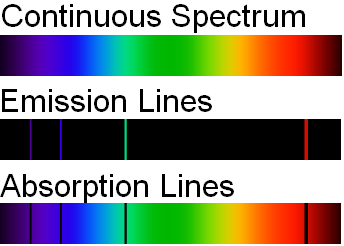
An emission line is formed when an atom or molecule makes a transition from a particular discrete energy level E₂ of an atom, to a lower energy level E₁, emitting a photon of a particular energy and wavelength. A spectrum of many such photons will show an emission spike at the wavelength associated with these photons.

An absorption line is formed when an atom or molecule makes a transition from a lower, E₁, to a higher discrete energy state, E₂, with a photon being absorbed in the process. These absorbed photons generally come from background continuum radiation (the full spectrum of electromagnetic radiation) and a spectrum will show a drop in the continuum radiation at the wavelength associated with the absorbed photons.

The two states must be bound states in which the electron is bound to the atom or molecule, so the transition is sometimes referred to as a "bound–bound" transition, as opposed to a transition in which the electron is ejected out of the atom completely ("bound–free" transition) into a continuum state, leaving an ionized atom, and generating continuum radiation.

A photon with an energy equal to the difference E₂ − E₁ between the energy levels is released or absorbed in the process. The frequency ν at which the spectral line occurs is related to the photon energy by Bohr's frequency condition E₂ − E₁ = hν where h denotes the Planck constant.^{[2][3][4][5][6][7]}

An atomic spectral line refers to emission and absorption events in a gas in which ${\displaystyle n_{2}}$ is the density of atoms in the upper-energy state for the line, and ${\displaystyle n_{1}}$ is the density of atoms in the lower-energy state for the line.

The emission of atomic line radiation at frequency ν may be described by an emission coefficient ${\displaystyle \varepsilon }$ with units of energy/(time × volume × solid angle). ε dt dV dΩ is then the energy emitted by a volume element ${\displaystyle dV}$ in time ${\displaystyle dt}$ into solid angle ${\displaystyle d\Omega }$. For atomic line radiation, $${\displaystyle \varepsilon ={\frac {h\nu }{4\pi }}n_{2}A_{21},}$$ where ${\displaystyle A_{21}}$ is the Einstein coefficient for spontaneous emission, which is fixed by the intrinsic properties of the relevant atom for the two relevant energy levels.

The absorption of atomic line radiation may be described by an absorption coefficient ${\displaystyle \kappa }$ with units of 1/length. The expression κ' dx gives the fraction of intensity absorbed for a light beam at frequency ν while traveling distance dx. The absorption coefficient is given by $${\displaystyle \kappa '={\frac {h\nu }{4\pi }}(n_{1}B_{12}-n_{2}B_{21}),}$$ where ${\displaystyle B_{12}}$ and ${\displaystyle B_{21}}$ are the Einstein coefficients for photon absorption and induced emission respectively. Like the coefficient ${\displaystyle A_{21}}$, these are also fixed by the intrinsic properties of the relevant atom for the two relevant energy levels. For thermodynamics and for the application of Kirchhoff's law, it is necessary that the total absorption be expressed as the algebraic sum of two components, described respectively by ${\displaystyle B_{12}}$ and ${\displaystyle B_{21}}$, which may be regarded as positive and negative absorption, which are, respectively, the direct photon absorption, and what is commonly called stimulated or induced emission.^[8][9][10]

The above equations have ignored the influence of the spectroscopic line shape. To be accurate, the above equations need to be multiplied by the (normalized) spectral line shape, in which case the units will change to include a 1/Hz term.

Under conditions of thermodynamic equilibrium, the number densities ${\displaystyle n_{2}}$ and ${\displaystyle n_{1}}$, the Einstein coefficients, and the spectral energy density provide sufficient information to determine the absorption and emission rates.

The number densities ${\displaystyle n_{2}}$ and ${\displaystyle n_{1}}$ are set by the physical state of the gas in which the spectral line occurs, including the local spectral radiance (or, in some presentations, the local spectral radiant energy density). When that state is either one of strict thermodynamic equilibrium, or one of so-called "local thermodynamic equilibrium",^[11][12][13] then the distribution of atomic states of excitation (which includes ${\displaystyle n_{2}}$ and ${\displaystyle n_{1}}$) determines the rates of atomic emissions and absorptions to be such that Kirchhoff's law of equality of radiative absorptivity and emissivity holds. In strict thermodynamic equilibrium, the radiation field is said to be black-body radiation and is described by Planck's law. For local thermodynamic equilibrium, the radiation field does not have to be a black-body field, but the rate of interatomic collisions must vastly exceed the rates of absorption and emission of quanta of light, so that the interatomic collisions entirely dominate the distribution of states of atomic excitation. Circumstances occur in which local thermodynamic equilibrium does not prevail, because the strong radiative effects overwhelm the tendency to the Maxwell–Boltzmann distribution of molecular velocities. For example, in the atmosphere of the Sun, the great strength of the radiation dominates. In the upper atmosphere of the Earth, at altitudes over 100 km, the rarity of intermolecular collisions is decisive.

In the cases of thermodynamic equilibrium and of local thermodynamic equilibrium, the number densities of the atoms, both excited and unexcited, may be calculated from the Maxwell–Boltzmann distribution, but for other cases, (e.g. lasers) the calculation is more complicated.

In 1916, Albert Einstein proposed that there are three processes occurring in the formation of an atomic spectral line. The three processes are referred to as spontaneous emission, stimulated emission, and absorption. With each is associated an Einstein coefficient, which is a measure of the probability of that particular process occurring. Einstein considered the case of isotropic radiation of frequency ν and spectral energy density ρ(ν).^{[3][14][15][16]} Paul Dirac derived the coefficients in a 1927 paper titled "The Quantum Theory of the Emission and Absorption of Radiation".^[17][18]

Hilborn has compared various formulations for derivations for the Einstein coefficients, by various authors.^[19] For example, Herzberg works with irradiance and wavenumber;^[20] Yariv works with energy per unit volume per unit frequency interval,^[21] as is the case in the more recent (2008) ^[22] formulation. Mihalas & Weibel-Mihalas work with radiance and frequency,^[13] as does Chandrasekhar,^[23] and Goody & Yung;^[24] Loudon uses angular frequency and radiance.^[25]

Spontaneous emission is the process by which an electron "spontaneously" (i.e. without any outside influence) decays from a higher energy level to a lower one. The process is described by the Einstein coefficient A₂₁ (s⁻¹), which gives the probability per unit time that an electron in state 2 with energy ${\displaystyle E_{2}}$ will decay spontaneously to state 1 with energy ${\displaystyle E_{1}}$, emitting a photon with an energy E₂ − E₁ = hν. Due to the energy-time uncertainty principle, the transition actually produces photons within a narrow range of frequencies called the spectral linewidth. If ${\displaystyle n_{i}}$ is the number density of atoms in state i , then the change in the number density of atoms in state 2 per unit time due to spontaneous emission will be $${\displaystyle \left({\frac {dn_{2}}{dt}}\right)_{\text{spontaneous}}=-A_{21}n_{2}.}$$

The same process results in an increase in the population of state 1: $${\displaystyle \left({\frac {dn_{1}}{dt}}\right)_{\text{spontaneous}}=A_{21}n_{2}.}$$

Stimulated emission (also known as induced emission) is the process by which an electron is induced to jump from a higher energy level to a lower one by the presence of electromagnetic radiation at (or near) the frequency of the transition. From the thermodynamic viewpoint, this process must be regarded as negative absorption. The process is described by the Einstein coefficient ${\displaystyle B_{21}}$ (m³ J⁻¹ s⁻²), which gives the probability per unit time per unit energy density of the radiation field per unit frequency that an electron in state 2 with energy ${\displaystyle E_{2}}$ will decay to state 1 with energy ${\displaystyle E_{1}}$, emitting a photon with an energy E₂ − E₁ = hν. The change in the number density of atoms in state 1 per unit time due to induced emission will be $${\displaystyle \left({\frac {dn_{1}}{dt}}\right)_{\text{neg. absorb.}}=B_{21}n_{2}\rho (\nu ),}$$ where ${\displaystyle \rho (\nu )}$ denotes the spectral energy density of the isotropic radiation field at the frequency of the transition (see Planck's law).

Stimulated emission is one of the fundamental processes that led to the development of the laser. Laser radiation is, however, very far from the present case of isotropic radiation.

Absorption is the process by which a photon is absorbed by the atom, causing an electron to jump from a lower energy level to a higher one. The process is described by the Einstein coefficient ${\displaystyle B_{12}}$ (m³ J⁻¹ s⁻²), which gives the probability per unit time per unit energy density of the radiation field per unit frequency that an electron in state 1 with energy ${\displaystyle E_{1}}$ will absorb a photon with an energy E₂ − E₁ = hν and jump to state 2 with energy ${\displaystyle E_{2}}$. The change in the number density of atoms in state 1 per unit time due to absorption will be $${\displaystyle \left({\frac {dn_{1}}{dt}}\right)_{\text{pos. absorb.}}=-B_{12}n_{1}\rho (\nu ).}$$

The Einstein coefficients are fixed probabilities per time associated with each atom, and do not depend on the state of the gas of which the atoms are a part. Therefore, any relationship that we can derive between the coefficients at, say, thermodynamic equilibrium will be valid universally.

At thermodynamic equilibrium, we will have a simple balancing, in which the net change in the number of any excited atoms is zero, being balanced by loss and gain due to all processes. With respect to bound-bound transitions, we will have detailed balancing as well, which states that the net exchange between any two levels will be balanced. This is because the probabilities of transition cannot be affected by the presence or absence of other excited atoms. Detailed balance (valid only at equilibrium) requires that the change in time of the number of atoms in level 1 due to the above three processes be zero: $${\displaystyle 0=A_{21}n_{2}+B_{21}n_{2}\rho (\nu )-B_{12}n_{1}\rho (\nu ).}$$

Along with detailed balancing, at temperature T we may use our knowledge of the equilibrium energy distribution of the atoms, as stated in the Maxwell–Boltzmann distribution, and the equilibrium distribution of the photons, as stated in Planck's law of black body radiation to derive universal relationships between the Einstein coefficients.

From Boltzmann distribution we have for the number of excited atomic species i: $${\displaystyle {\frac {n_{i}}{n}}={\frac {g_{i}e^{-E_{i}/kT}}{Z}},}$$ where n is the total number density of the atomic species, excited and unexcited, k is the Boltzmann constant, T is the temperature, ${\displaystyle g_{i}}$ is the degeneracy (also called the multiplicity) of state i, and Z is the partition function. From Planck's law of black-body radiation at temperature T we have for the spectral radiance (radiance is energy per unit time per unit solid angle per unit projected area, when integrated over an appropriate spectral interval)^[26] at frequency ν $${\displaystyle \rho _{\nu }(\nu ,T)=F(\nu ){\frac {1}{e^{h\nu /kT}-1}},}$$ where^[27] $${\displaystyle F(\nu )={\frac {2h\nu ^{3}}{c^{3}}},}$$ where ${\displaystyle c}$ is the speed of light and ${\displaystyle h}$ is the Planck constant.

Substituting these expressions into the equation of detailed balancing and remembering that E₂ − E₁ = hν yields $${\displaystyle A_{21}g_{2}e^{-h\nu /kT}+B_{21}g_{2}e^{-h\nu /kT}{\frac {F(\nu )}{e^{h\nu /kT}-1}}=B_{12}g_{1}{\frac {F(\nu )}{e^{h\nu /kT}-1}},}$$ or $${\displaystyle A_{21}g_{2}(1-e^{-h\nu /kT})+B_{21}g_{2}F(\nu )e^{-h\nu /kT}=B_{12}g_{1}F(\nu ).}$$

The above equation must hold at any temperature, so from ${\displaystyle T\to \infty }$ one gets $${\displaystyle B_{21}g_{2}=B_{12}g_{1},}$$ and from ${\displaystyle T\to 0}$ $${\displaystyle A_{21}g_{2}=B_{21}g_{2}F(\nu ).}$$

Therefore, the three Einstein coefficients are interrelated by $${\displaystyle {\frac {A_{21}}{B_{21}}}=F(\nu )}$$ and $${\displaystyle {\frac {B_{21}}{B_{12}}}={\frac {g_{1}}{g_{2}}}.}$$

When this relation is inserted into the original equation, one can also find a relation between ${\displaystyle A_{21}}$ and ${\displaystyle B_{12}}$, involving Planck's law.

The oscillator strength ${\displaystyle f_{12}}$ is defined by the following relation to the cross section ${\displaystyle \sigma }$ for absorption:^[19] $${\displaystyle \sigma ={\frac {e^{2}}{4\varepsilon _{0}m_{e}c}}\,f_{12}\,\phi _{\nu }={\frac {\pi e^{2}}{2\varepsilon _{0}m_{e}c}}\,f_{12}\,\phi _{\omega },}$$

where ${\displaystyle e}$ is the electron charge, ${\displaystyle m_{e}}$ is the electron mass, and ${\displaystyle \phi _{\nu }}$ and ${\displaystyle \phi _{\omega }}$ are normalized distribution functions in frequency and angular frequency respectively. This allows all three Einstein coefficients to be expressed in terms of the single oscillator strength associated with the particular atomic spectral line: $${\displaystyle {\begin{aligned}B_{12}&={\frac {e^{2}}{4\varepsilon _{0}m_{e}h\nu }}f_{12},\\[1ex]B_{21}&={\frac {e^{2}}{4\varepsilon _{0}m_{e}h\nu }}{\frac {g_{1}}{g_{2}}}f_{12},\\[1ex]A_{21}&={\frac {2\pi \nu ^{2}e^{2}}{\varepsilon _{0}m_{e}c^{3}}}{\frac {g_{1}}{g_{2}}}f_{12}.\end{aligned}}}$$

The value of A and B coefficients can be calculated using quantum mechanics where dipole approximations in time dependent perturbation theory is used. While the calculation of B coefficient can be done easily, that of A coefficient requires using results of second quantization. This is because the theory developed by dipole approximation and time dependent perturbation theory gives a semiclassical description of electronic transition which goes to zero as perturbing fields go to zero. The A coefficient which governs spontaneous emission should not go to zero as perturbing fields go to zero. The result for transition rates of different electronic levels as a result of spontaneous emission is given as (in SI units):^[28][19][29] $${\displaystyle w_{i\to f}^{\text{s.emi}}={\frac {\omega _{if}^{3}e^{2}}{3\pi \varepsilon _{0}\hbar c^{3}}}\left|\langle f|{\vec {r}}|i\rangle \right|^{2}=A_{if}}$$

For B coefficient, straightforward application of dipole approximation in time dependent perturbation theory yields (in SI units):^[30][29] $${\displaystyle w_{i\rightarrow f}^{\text{abs}}={\frac {u(\omega _{fi})\pi e^{2}}{3\varepsilon _{0}\hbar ^{2}}}\left|\langle f|{\vec {r}}|i\rangle \right|^{2}=B_{if}^{\text{abs}}u(\omega _{fi})}$$ $${\displaystyle w_{i\to f}^{\text{emi}}={\frac {u(\omega _{if})\pi e^{2}}{3\varepsilon _{0}\hbar ^{2}}}\left|\langle f|{\vec {r}}|i\rangle \right|^{2}=B_{if}^{emi}u(\omega _{if})}$$

Note that the rate of transition formula depends on dipole moment operator. For higher order approximations, it involves quadrupole moment and other similar terms.

Here, the B coefficients are chosen to correspond to ${\displaystyle \omega }$ energy distribution function. Often these different definitions of B coefficients are distinguished by superscript, for example, ${\textstyle B_{21}^{f}={\frac {B_{21}^{\omega }}{2\pi }}}$ where ${\textstyle B_{21}^{f}}$ term corresponds to frequency distribution and ${\textstyle B_{21}^{\omega }}$ term corresponds to ${\displaystyle \omega }$ distribution.^[19] The formulas for B coefficients varies inversely to that of the energy distribution chosen, so that the transition rate is same regardless of convention.

Hence, AB coefficients are calculated using dipole approximation as: $${\displaystyle {\begin{aligned}A_{ab}&={\frac {\omega _{ab}^{3}e^{2}}{3\pi \varepsilon _{0}\hbar c^{3}}}\left|\langle a|{\vec {r}}|b\rangle \right|^{2}\\[1ex]B_{ab}&={\frac {\pi e^{2}}{3\varepsilon _{0}\hbar ^{2}}}\left|\langle a|{\vec {r}}|b\rangle \right|^{2}\end{aligned}}}$$ where ${\displaystyle \omega _{ab}={\frac {E_{a}-E_{b}}{\hbar }}}$ and B coefficients correspond to ${\displaystyle \omega }$ energy distribution function.

Hence the following ratios are also derived: $${\displaystyle {\frac {B_{12}}{B_{21}}}=1}$$ and $${\displaystyle {\frac {A_{if}}{B}}={\frac {\omega _{if}^{3}\hbar }{\pi ^{2}c^{3}}}}$$

It follows from theory that:^[29] $${\displaystyle {\frac {dN_{b}}{dt}}=-A_{ba}N_{b}-N_{b}u(\omega _{ba})B_{ba}+N_{a}u(\omega _{ba})B_{ab}=-N_{b}w_{b\to a}^{\text{s.emi}}-N_{b}w_{b\to a}^{\text{emi}}+N_{a}w_{a\to b}^{\text{abs}}}$$ where ${\displaystyle N_{a}}$ and ${\displaystyle N_{b}}$ are number of occupied energy levels of ${\displaystyle E_{a}}$ and ${\displaystyle E_{b}}$ respectively, where ${\displaystyle E_{b}>E_{a}}$. Note that from time dependent perturbation theory application, the fact that only radiation whose ${\displaystyle \omega }$ is close to value of ${\displaystyle \omega _{ba}}$ can produce respective stimulated emission or absorption, is used.

Where Maxwell distribution involving ${\displaystyle N_{a}}$ and ${\displaystyle N_{b}}$ ensures ${\displaystyle {\frac {N_{a}}{N_{b}}}={\frac {e^{-E_{a}\beta }}{e^{-E_{b}\beta }}}=e^{\omega _{ba}\hbar \beta }}$

Solving for ${\displaystyle u}$ for equilibrium condition ${\displaystyle {\frac {dN_{b}}{dt}}=0}$ using the above equations and ratios while generalizing ${\displaystyle \omega _{ba}}$ to ${\displaystyle \omega }$, we get: $${\displaystyle u_{\omega }(\omega ,T)={\frac {\omega ^{3}\hbar }{\pi ^{2}c^{3}}}{\frac {1}{e^{\omega \hbar \beta }-1}}}$$ which is the angular frequency energy distribution from Planck's law.^[29]