
Community hub
Recent from talks
Contribute something
Nothing was collected or created yet.
Coronal loop
View on WikipediaThis article needs additional citations for verification. (March 2022) |

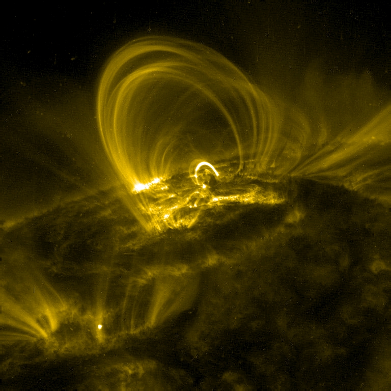
In solar physics, a coronal loop is a well-defined arch-like structure in the Sun's atmosphere made up of relatively dense plasma confined and isolated from the surrounding medium by magnetic flux tubes. Coronal loops begin and end at two footpoints on the photosphere and project into the transition region and lower corona. They typically form and dissipate over periods of seconds to days[1] and may span anywhere from 1 to 1,000 megametres (621 to 621,000 mi) in length.[2]
Coronal loops are often associated with the strong magnetic fields located within active regions and sunspots. The number of coronal loops varies with the 11 year solar cycle.
Origin and physical features
[edit]Due to a natural process called the solar dynamo driven by heat produced in the Sun's core, convective motion of the electrically conductive plasma which makes up the Sun creates electric currents, which in turn create powerful magnetic fields in the Sun's interior. These magnetic fields are in the form of closed loops of magnetic flux, which are twisted and tangled by solar differential rotation (the different rotation rates of the plasma at different latitudes of the solar sphere). A coronal loop occurs when a curved arc of the magnetic field projects through the visible surface of the Sun, the photosphere, protruding into the solar atmosphere.
Within a coronal loop, the paths of the moving electrically charged particles which make up its plasma—electrons and ions—are sharply bent by the Lorentz force when moving transverse to the loop's magnetic field. As a result, they can only move freely parallel to the magnetic field lines, tending to spiral around these lines. Thus, the plasma within a coronal loop cannot escape sideways out of the loop and can only flow along its length. This is known as the frozen-in condition.[3]
The strong interaction of the magnetic field with the dense plasma on and below the Sun's surface tends to tie the magnetic field lines to the motion of the Sun's plasma; thus, the two footpoints (the location where the loop enters the photosphere) are anchored to and rotate with the Sun's surface. Within each footpoint, the strong magnetic flux tends to inhibit the convection currents which carry hot plasma from the Sun's interior to the surface, so the footpoints are often (but not always) cooler than the surrounding photosphere. These appear as dark spots on the Sun's surface, known as sunspots. Thus, sunspots tend to occur under coronal loops, and tend to come in pairs of opposite magnetic polarity; a point where the magnetic field loop emerges from the photosphere is a North magnetic pole, and the other where the loop enters the surface again is a South magnetic pole.
Coronal loops form in a wide range of sizes, from the minimum observable scale (< 100 km) to 10,000 km. There is currently no accepted theory of what defines the edge of a loop, which is embedded in a general corona that is itself strongly magnetized. Coronal loops have a wide variety of temperatures along their lengths. Loops at temperatures below 1 megakelvin (MK) are generally known as cool loops; those existing at around 1 MK are known as warm loops; and those beyond 1 MK are known as hot loops. Naturally, these different categories radiate at different wavelengths.[4]
A related phenomenon is the open flux tube, in which magnetic fields extend from the surface far into the corona and heliosphere; these are the source of the Sun's large scale magnetic field (magnetosphere) and the solar wind.
-
 A diagram showing the evolution of the solar magnetic flux over one solar cycle
 -
 Diagram of the low corona and transition region, where many scales of coronal loops can be observed
 -
 A modelled example of a quiescent coronal loop (energy contributions)


Location
[edit]Coronal loops have been shown on both active and quiet regions of the solar surface. Active regions on the solar surface take up small areas but produce the majority of activity and are often the source of flares and coronal mass ejections due to the intense magnetic field present. Active regions produce 82% of the total coronal heating energy.[5][6]
Dynamic flows
[edit]Many solar observation missions have observed strong plasma flows and highly dynamic processes in coronal loops. For example, SUMER observations suggest flow velocities of 5–16 km/s in the solar disk, and other joint SUMER/TRACE observations detect flows of 15–40 km/s.[7][8] Very high plasma velocities (in the range of 40–60 km/s) have been detected by the Flat Crystal Spectrometer (FCS) on board the Solar Maximum Mission.
History of observations
[edit]Before 1991
[edit]Despite progress made by ground-based telescopes and eclipse observations of the corona, space-based observations became necessary to escape the obscuring effect of the Earth's atmosphere. Rocket missions such as the Aerobee flights and Skylark rockets successfully measured solar extreme ultraviolet (EUV) and X-ray emissions. However, these rocket missions were limited in lifetime and payload. Later, satellites such as the Orbiting Solar Observatory series (OSO-1 to OSO-8), Skylab, and the Solar Maximum Mission (the first observatory to last the majority of a solar cycle: from 1980 to 1989) were able to gain far more data across a much wider range of emission.[9][10]
1991–present day
[edit]
In August 1991, the solar observatory spacecraft Yohkoh launched from the Kagoshima Space Center. During its 10 years of operation, it revolutionized X-ray observations. Yohkoh carried four instruments; of particular interest is the SXT instrument, which observed X-ray-emitting coronal loops. This instrument observed X-rays in the 0.25–4.0 keV range, resolving solar features to 2.5 arc seconds with a temporal resolution of 0.5–2 seconds. SXT was sensitive to plasma in the 2–4 MK temperature range, making its data ideal for comparison with data later collected by TRACE of coronal loops radiating in the extra ultraviolet (EUV) wavelengths.[11]
The next major step in solar physics came in December 1995, with the launch of the Solar and Heliospheric Observatory (SOHO) from Cape Canaveral Air Force Station. SOHO originally had an operational lifetime of two years. The mission was extended to March 2007 due to its resounding success, allowing SOHO to observe a complete 11-year solar cycle. SOHO has 12 instruments on board, all of which are used to study the transition region and corona. In particular, the Extreme ultraviolet Imaging Telescope (EIT) instrument is used extensively in coronal loop observations. EIT images the transition region through to the inner corona by using four band passes—171 Å FeIX, 195 Å FeXII, 284 Å FeXV, and 304 Å HeII, each corresponding to different EUV temperatures—to probe the chromospheric network to the lower corona.
In April 1998, the Transition Region and Coronal Explorer (TRACE) was launched from Vandenberg Air Force Base. Its observations of the transition region and lower corona, made in conjunction with SOHO, give an unprecedented view of the solar environment during the rising phase of the solar maximum, an active phase in the solar cycle. Due to the high spatial (1 arc second) and temporal resolution (1–5 seconds), TRACE has been able to capture highly detailed images of coronal structures, whilst SOHO provides the global (lower resolution) picture of the Sun. This campaign demonstrates the observatory's ability to track the evolution of steady-state (or 'quiescent') coronal loops. TRACE uses filters sensitive to various types of electromagnetic radiation; in particular, the 171 Å, 195 Å, and 284 Å band passes are sensitive to the radiation emitted by quiescent coronal loops.
See also
[edit]References
[edit]- ^ Loff, Sarah (2015-04-17). "Coronal Loops in an Active Region of the Sun". NASA. Retrieved 2022-03-28.
- ^ Reale, Fabio (July 2014). "Coronal Loops: Observations and Modeling of Confined Plasma" (PDF). Living Reviews in Solar Physics. 11 (4): 4. Bibcode:2014LRSP...11....4R. doi:10.12942/lrsp-2014-4. PMC 4841190. PMID 27194957. Retrieved 16 March 2022.
- ^ Malanushenko, A.; Cheung, M. C. M.; DeForest, C. E.; Klimchuk, J. A.; Rempel, M. (1 March 2022). "The Coronal Veil". The Astrophysical Journal. 927 (1): 1. arXiv:2106.14877. Bibcode:2022ApJ...927....1M. doi:10.3847/1538-4357/ac3df9. S2CID 235658491.
- ^ Vourlidas, A.; J. A. Klimchuk; C. M. Korendyke; T. D. Tarbell; B. N. Handy (2001). "On the correlation between coronal and lower transition region structures at arcsecond scales". Astrophysical Journal. 563 (1): 374–380. Bibcode:2001ApJ...563..374V. CiteSeerX 10.1.1.512.1861. doi:10.1086/323835. S2CID 53124376.
- ^ Aschwanden, M. J. (2001). "An evaluation of coronal heating models for Active Regions based on Yohkoh, SOHO, and TRACE observations". Astrophysical Journal. 560 (2): 1035–1044. Bibcode:2001ApJ...560.1035A. doi:10.1086/323064. S2CID 121226839.
- ^ Aschwanden, M. J. (2004). Physics of the Solar Corona. An Introduction. Praxis Publishing Ltd. ISBN 978-3-540-22321-4.
- ^ Spadaro, D.; A. C. Lanzafame; L. Consoli; E. Marsch; D. H. Brooks; J. Lang (2000). "Structure and dynamics of an active region loop system observed on the solar disc with SUMER on SOHO". Astronomy & Astrophysics. 359: 716–728. Bibcode:2000A&A...359..716S.
- ^ Winebarger, A. R.; H. Warren; A. van Ballegooijen; E. E. DeLuca; L. Golub (2002). "Steady flows detected in extreme-ultraviolet loops". Astrophysical Journal Letters. 567 (1): L89 – L92. Bibcode:2002ApJ...567L..89W. doi:10.1086/339796.
- ^ Vaiana, G. S.; J. M. Davis; R. Giacconi; A. S. Krieger; J. K. Silk; A. F. Timothy; M. Zombeck (1973). "X-Ray Observations of Characteristic Structures and Time Variations from the Solar Corona: Preliminary Results from SKYLAB". Astrophysical Journal Letters. 185: L47 – L51. Bibcode:1973ApJ...185L..47V. doi:10.1086/181318.
- ^ Strong, K. T.; J. L. R. Saba; B. M. Haisch; J. T. Schmelz (1999). The many faces of the Sun: a summary of the results from NASA's Solar Maximum Mission. New York: Springer.
{{cite book}}: CS1 maint: publisher location (link) - ^ Aschwanden, M. J. (2002). "Observations and models of coronal loops: From Yohkoh to TRACE, in Magnetic coupling of the solar atmosphere". 188: 1–9.
{{cite journal}}: Cite journal requires|journal=(help)
External links
[edit]- TRACE homepage
- Solar and Heliospheric Observatory, including near-real-time images of the solar corona
- Coronal heating problem at Innovation Reports
- NASA/GSFC description of the coronal heating problem
- FAQ about coronal heating
- Animated explanation of Coronal loops and their role in creating Prominences Archived 2015-11-16 at the Wayback Machine (University of South Wales)
| National | |
|---|---|
| Other | |
Coronal loop
View on GrokipediaFundamentals
Definition and overview
Coronal loops are bright, arch-like structures in the Sun's corona, consisting of dense plasma confined and guided along closed magnetic field lines that connect regions of opposite polarity on the solar surface. These loops typically form above active regions and sunspots, serving as the fundamental building blocks of the X-ray and extreme ultraviolet (EUV) bright corona by channeling and isolating hot plasma from the surrounding environment.[5][3] In terms of scale, coronal loops exhibit a wide range of dimensions, with heights or semi-lengths typically spanning 5,000 to 100,000 km, widths of 1,000 to 10,000 km, and lifetimes from minutes to several days, depending on their association with solar activity such as flares. Their visibility in EUV and X-ray wavelengths arises from the high temperatures of the confined plasma, which range from 1 to 20 million K—far exceeding the roughly 6,000 K of the underlying photosphere—allowing them to emit strongly through thermal bremsstrahlung and line radiation.[5][6] The plasma within coronal loops is primarily composed of fully ionized hydrogen and helium, behaving as an ideal, low-beta gas that closely follows the magnetic field lines due to the dominance of magnetic forces over gas pressure. This confinement maintains the loops' structure and enables efficient energy transport along the field, highlighting their central role in the dynamic equilibrium of the solar atmosphere.[5]Physical characteristics
Coronal loops typically exhibit a semicircular or fan-like geometry, particularly within active regions, where multiple loops may form arcades fanning out from magnetic concentrations. These structures are anchored at their footpoints in the photosphere or chromosphere, with lengths ranging from approximately 10,000 to 200,000 km and cross-sections that remain roughly constant along their extent, deviating from perfect circularity by less than 30%.[7] The temperature structure of coronal loops often features a monotonic increase from cooler footpoints to a hotter apex, reflecting hydrostatic equilibrium and heating patterns. In typical active region loops, footpoint temperatures are around 1 MK, rising to apex values of 3–10 MK for hot loops, though many observed loops show nearly isothermal profiles with minimal gradients along their length. Loops are frequently multi-thermal, comprising strands or components with a broad temperature distribution spanning 1–20 MK, as revealed by differential emission measure analyses, indicating unresolved finer structures or dynamic evolution.[8][7] Electron density profiles in coronal loops decrease with height from the footpoints, typically ranging from to cm in bright quiescent loops, with higher values up to cm during flares. This variation is quantified using emission measure, defined as the integral of the square of the electron density along the line of sight, which peaks in the 2–10 MK range for active region loops and helps map density distributions non-uniformly across multi-thermal structures.[7][9] Brightness in coronal loops arises from thermal emission, with significant variations observed in X-ray (for hot plasma >2 MK) and extreme ultraviolet (EUV) wavelengths (for warmer plasma ~1 MK). Cooler loops, with temperatures below 1 MK, are prominent in the transition region and appear in EUV bands, contributing to the overall multi-thermal emission profile and highlighting density enhancements in lower-temperature components.[7]Formation and dynamics
Magnetic origins
Coronal loops originate from the emergence of magnetic flux from the solar interior, where convective motions buoy up twisted magnetic flux tubes through the convection zone to the photosphere, forming bipolar magnetic regions in active regions. This process, first described by magnetic buoyancy principles, drives the initial structuring of loops as arched field lines piercing the surface.[10] Subsequent magnetic reconnection between emerging flux and pre-existing coronal fields refines the loop topology, connecting opposite polarity footpoints and confining plasma along closed field lines.[11] The magnetic field strength in coronal loops typically ranges from 10 to 100 Gauss at the photospheric footpoints, where intense concentrations anchor the structures, and weakens to 1 to 10 Gauss along the coronal apex due to flux expansion. Twisted flux tubes play a crucial role in this configuration, providing the helicity that stabilizes loops against rapid disruption while enabling gradual evolution through differential rotation and shearing.[1] Coronal loops are most prevalent during solar maximum, when enhanced flux emergence populates active regions with sunspots and surrounding plages, amplifying the density of bipolar structures. These features diminish toward solar minimum as active region formation wanes, linking loop abundance directly to the 11-year solar cycle dynamics.[12] Topologically, coronal loops represent closed magnetic field lines that trap plasma in the hot corona, contrasting with open field lines in coronal holes where solar wind escapes freely. In prominences, loops often manifest as arcade structures, with multiple aligned arches supporting cool filamentary material against the overarching field.Plasma flows and heating
Siphon flows in coronal loops arise from pressure differences between the two footpoints, resulting in asymmetric plasma motion along the loop from the higher-pressure end to the lower-pressure end.[13] These flows, guided by the magnetic field lines, can reach speeds up to 100 km/s and are typically subsonic or supersonic depending on the loop geometry and heating asymmetry.[14] The high temperatures in coronal loops, often exceeding 10^6 K, require continuous heating to balance energy losses. One prominent mechanism is nanoflare heating, involving numerous small-scale magnetic reconnection events that release energy impulsively.[15] Each nanoflare deposits approximately 10^{24} to 10^{26} erg, collectively maintaining the loop's thermal structure through repeated occurrences.[15] An alternative is wave heating driven by Alfvén waves, which propagate along the loop and dissipate energy via turbulence or resonant absorption, contributing to the overall energy input.[16] The energy balance in coronal loops is governed by the equation where is the internal energy density, is the volumetric heating rate, represents radiative losses given by with erg cm s at coronal temperatures around 10^6 K, and denotes conductive losses described by the flux with .[17] This balance ensures quasi-static equilibrium, with heating countering the dominant losses from radiation and conduction along the loop.[17] Heating events in coronal loops trigger chromospheric evaporation, where intense energy deposition heats chromospheric plasma, driving upflows that fill the loop with hot material.[18] These upflows, often observed at speeds of 10–20 km/s near the footpoints and decreasing with height, replenish the coronal density and sustain the loop's structure.[18]Observations
Early detections
Early observations of the solar corona, primarily conducted from the ground during total solar eclipses, began revealing structured, loop-like features in white light as early as the 1940s. These photographs captured arch-like extensions and streamers emanating from the solar limb, interpreted as plasma confined along magnetic field lines in the corona.[19] Coronagraphs, developed by Bernard Lyot in the 1930s and deployed at observatories like Pic du Midi in the 1940s and 1950s, enabled routine imaging of the corona without waiting for eclipses, further highlighting these elongated, curved structures amid the fainter diffuse emission.[20] By the 1960s, eclipse and coronagraph data had established that such features varied with solar activity, often appearing brighter near active regions.[5] Pioneering space-based detections in the 1960s came from suborbital rocket flights equipped with grazing-incidence X-ray telescopes, which first imaged the corona in soft X-rays. A landmark flight on June 8, 1968, captured high-resolution X-ray photographs during a solar flare, revealing bright, arched structures interconnecting active regions—early evidence of hot coronal loops emitting at temperatures exceeding 10 million Kelvin.[21] Subsequent rocket missions in the late 1960s and early 1970s confirmed these loop-like emissions as persistent features of the quiescent corona, not just flares, with X-ray brightness concentrated above magnetically complex areas.[22] Theoretical groundwork for understanding these structures emerged in the late 1950s, when Eugene Parker highlighted the "coronal heating problem"—the enigma of how the corona reaches million-degree temperatures despite cooling by expansion into the solar wind. Parker argued that localized structures like loops could facilitate energy transport from the photosphere, channeling magnetic energy to heat confined plasma volumes. This framework underscored the need for loop observations to resolve the energy balance. The Skylab mission (1973–1974) marked a breakthrough with its Apollo Telescope Mount (ATM), delivering the first prolonged X-ray imaging of the corona via instruments like the S-054 X-ray telescope, which produced over 32,000 images.[5] These revealed intricate networks of hot, bright loops spanning active regions, with temperatures up to 3–5 million Kelvin and lengths of hundreds of thousands of kilometers.[23] Skylab also discovered "loop prominences," cool, dense plasma threads suspended along these hot X-ray loops, providing initial insights into multi-temperature plasma dynamics within coronal structures.[24]Modern imaging and data
The Yohkoh mission, operational from 1991 to 2001, marked a significant advancement in coronal loop observations through its Soft X-ray Telescope (SXT), which achieved a resolution of approximately 2.5 arcseconds, enabling the first detailed imaging of loop fine structure in soft X-rays.[25] This instrument revealed the arch-like morphology and internal threading of loops within active regions, distinguishing between bright, hot plasma confined in magnetic flux tubes and surrounding diffuse emission.[26] A key discovery from SXT data was the identification of cooling flows in coronal loops, where plasma cools radiatively while draining along field lines, providing evidence of dynamic thermal evolution in quasi-steady structures.[25] The Transition Region and Coronal Explorer (TRACE), launched in 1998 and operational until 2010, introduced high-resolution extreme ultraviolet (EUV) imaging at 1 arcsecond resolution, targeting cooler loops formed at temperatures around 1 million Kelvin.[27] TRACE's observations highlighted the intricate, filamentary substructure of these loops, often resolving individual threads within larger arches and capturing their evolution over timescales of minutes to hours.[28] Complementing this, the Hinode mission, launched in 2006 and ongoing, employs the Extreme-ultraviolet Imaging Spectrometer (EIS) to measure Doppler shifts in emission lines, quantifying plasma flows along loops with velocities up to 100 km/s.[29] EIS data have demonstrated bidirectional flows in loop legs, with blue shifts indicating upflows and red shifts downflows, offering direct spectroscopic evidence of mass circulation driven by heating imbalances.[30] More recent missions have further enhanced multi-wavelength coverage and proximity measurements. The Solar Dynamics Observatory (SDO), launched in 2010 and still active, uses the Atmospheric Imaging Assembly (AIA) to produce time-series movies across seven EUV and two UV channels, resolving loop dynamics at 0.6 arcsecond resolution and 12-second cadence.[31] These observations capture the multi-thermal nature of loops, showing how plasma at different temperatures (0.5–20 million Kelvin) threads the same magnetic structure, and enable tracking of eruptions and reconnections in real time.[32] The Parker Solar Probe, launched in 2018 and continuing operations, provides the first in-situ measurements within 20 solar radii (and as low as ~8.5 solar radii as of 2024), sampling plasma and magnetic fields in the inner corona associated with coronal magnetic structures including those near loop tops and open field regions.[33] Its data reveal high-beta plasma environments consistent with coronal conditions, including switchbacks and energetic particles indicative of reconnection processes.[34] The Solar Orbiter mission, launched in 2020 and operational as of 2025, complements these efforts with its Extreme Ultraviolet Imager (EUI), providing high-resolution EUV images at 1 arcsecond resolution or better, enabling stereoscopic observations of coronal loops in conjunction with SDO. These observations have revealed nearly circular cross-sections of loops, temporally coherent intensity variations, and persistent magnetic reconnection in medium-sized loops, enhancing understanding of their three-dimensional morphology and dynamics.[35][36] Key findings from these missions include evidence of nanoflares as a heating mechanism, with 2012 SDO/AIA observations detecting impulsive brightenings in loop footpoints that release energy equivalent to 10^24–10^25 ergs, sufficient to maintain coronal temperatures without large-scale flares.[37] Additionally, TRACE data from the late 1990s provided the first detections of loop oscillations, observing transverse kink modes with periods of 2–5 minutes and damping times of about 10 minutes, interpreted as magnetohydrodynamic waves propagating along loop waveguides.[38]Theoretical models
Equilibrium and stability
Coronal loops achieve hydrostatic equilibrium when the downward gravitational force on the plasma is balanced by the upward pressure gradient along the loop's curved structure. In static models, this balance is coupled with energy considerations, where heating is offset by radiative cooling and thermal conduction. The seminal Rosner-Tucker-Vaiana (RTV) scaling laws, derived from steady-state solutions assuming uniform heating and neglecting flows, relate the maximum temperature to the base pressure and loop semi-length via (in cgs units), while the heating rate scales as .[39] These relations highlight how conduction dominates energy transport in hot loops, with radiation more significant in cooler segments, providing a foundational framework for understanding loop energetics.[39] Magnetohydrodynamic (MHD) equilibrium in coronal loops requires the Lorentz force to balance plasma pressure gradients and gravity, often approximated under low- conditions where magnetic tension dominates. Force-free fields, satisfying , represent ideal configurations where the current is parallel to the magnetic field, minimizing magnetic stress while supporting loop topology.[40] For linear force-free models with uniform , analytical solutions in cylindrical geometry describe twisted flux tubes that align with observed loop shears, enabling extrapolation from photospheric magnetograms to coronal heights. These models capture the helical structure essential for loop stability, with quantifying the twist level. Stability analyses reveal thresholds beyond which loops become susceptible to resistive MHD instabilities. The kink mode, an ideal or resistive instability driven by excessive magnetic twist, sets in when the twist angle exceeds approximately for line-tied loops, leading to helical deformations that can trigger reconnection and energy release.[41] Similarly, the ballooning instability arises from pressure-driven perturbations in curved field lines, with a critical loop length (where is the radius of curvature) marking the onset for interchange-like modes in high- segments.[42] These criteria underscore the role of line-tying at photospheric footpoints in enhancing stability compared to uniform plasmas.[41] Numerical simulations of loop equilibrium often employ one-dimensional hydrodynamic models along the field line, solving the energy equation to capture time-dependent balances between enthalpy flux, heating , radiative losses , and conductive flux .[43] Early implementations, such as those incorporating RTV assumptions, demonstrate how impulsive heating leads to quasi-static states, with conduction smoothing temperature profiles over timescales of minutes.[43] These models validate scaling laws against observed loop parameters, like densities around cm and temperatures up to 10 MK, while revealing deviations due to non-uniform heating.[43]Oscillations and waves
Coronal loops exhibit a variety of magnetohydrodynamic (MHD) oscillations, which are transverse or longitudinal displacements driven by impulsive events such as flares or jets. These oscillations are classified into fast and slow magnetoacoustic modes. Fast magnetoacoustic kink modes, characterized by periods of 1–5 minutes and phase speeds ranging from 100 to 1000 km/s, involve the lateral displacement of the entire loop cross-section and are the most commonly observed type in extreme ultraviolet (EUV) imaging.[44] Slow sausage modes, in contrast, feature radial pulsations with compression and rarefaction along the loop axis, typically propagating at speeds near the local sound speed of about 100–200 km/s in coronal plasma.[45] Coronal seismology leverages these oscillations to diagnose loop properties noninvasively. The kink speed provides estimates of the loop radius and magnetic field strength via the thin-tube approximation:where is the magnetic field, is the vacuum permeability, and is the internal plasma density (often termed the "mantle" density in loop models). By measuring the oscillation period and loop length (where ), researchers infer values typically around 5–20 G in active region loops. This approach has been validated through comparisons with potential field extrapolations from photospheric magnetograms.[46] Damping of these oscillations occurs rapidly, often within 2–3 cycles, limiting their visibility. The primary mechanism for kink modes is resonant absorption, where wave energy transfers to the loop boundary layer due to spatial gradients in the Alfvén speed across the density contrast between the loop interior and external corona. Non-ideal MHD effects, such as finite resistivity, contribute additional damping by enabling Ohmic dissipation in thin current sheets at the resonant surface, with damping rates scaling inversely with the resistivity parameter.[47] Recent observations from the Solar Dynamics Observatory (SDO) in the 2020s have revealed decaying kink oscillations triggered post-flare, with decay times of 5–15 minutes and amplitudes up to 1–5 Mm, often coexisting with decayless regimes in multi-stranded loops.[48] These findings highlight the role of kink waves in coronal heating, where dissipated energy contributes to maintaining loop temperatures around 1–2 MK; the associated energy flux is estimated as , with the wave amplitude velocity (typically 5–50 km/s), yielding fluxes of 10–200 erg cm⁻² s⁻¹ sufficient to balance radiative losses in quiet active regions.
References
- https://solarscience.msfc.[nasa](/page/NASA).gov/feature3.shtml