
Community hub
Recent from talks
Contribute something
Nothing was collected or created yet.
Discounting
View on WikipediaIn finance, discounting is a mechanism in which a debtor obtains the right to delay payments to a creditor, for a defined period of time, in exchange for a charge or fee.[1] Essentially, the party that owes money in the present purchases the right to delay the payment until some future date.[2] This transaction is based on the fact that most people prefer current interest to delayed interest because of mortality effects, impatience effects, and salience effects.[3] The discount, or charge, is the difference between the original amount owed in the present and the amount that has to be paid in the future to settle the debt.[1]
The discount is usually associated with a discount rate, which is also called the discount yield.[1][2][4] The discount yield is the proportional share of the initial amount owed (initial liability) that must be paid to delay payment for 1 year.

Since a person can earn a return on money invested over some period of time, most economic and financial models assume the discount yield is the same as the rate of return the person could receive by investing this money elsewhere (in assets of similar risk) over the given period of time covered by the delay in payment.[1][2][5] The concept is associated with the opportunity cost of not having use of the money for the period of time covered by the delay in payment. The relationship between the discount yield and the rate of return on other financial assets is usually discussed in economic and financial theories involving the inter-relation between various market prices, and the achievement of Pareto optimality through the operations in the capitalistic price mechanism,[2] as well as in the discussion of the efficient (financial) market hypothesis.[1][2][6] The person delaying the payment of the current liability is essentially compensating the person to whom he/she owes money for the lost revenue that could be earned from an investment during the time period covered by the delay in payment.[1] Accordingly, it is the relevant "discount yield" that determines the "discount", and not the other way around.
As indicated, the rate of return is usually calculated in accordance to an annual return on investment. Since an investor earns a return on the original principal amount of the investment as well as on any prior period investment income, investment earnings are "compounded" as time advances.[1][2] Therefore, considering the fact that the "discount" must match the benefits obtained from a similar investment asset, the "discount yield" must be used within the same compounding mechanism to negotiate an increase in the size of the "discount" whenever the time period of the payment is delayed or extended.[2][6] The "discount rate" is the rate at which the "discount" must grow as the delay in payment is extended.[7] This fact is directly tied into the time value of money and its calculations.[1]

The "time value of money" indicates there is a difference between the "future value" of a payment and the "present value" of the same payment. The rate of return on investment should be the dominant factor in evaluating the market's assessment of the difference between the future value and the present value of a payment; and it is the market's assessment that counts the most.[6] Therefore, the "discount yield", which is predetermined by a related return on investment that is found in the different markets in the financial sector, is what is used within the time-value-of-money calculations to determine the "discount" required to delay payment of a financial liability for a given period of time.
Basic calculation
[edit]If we consider the value of the original payment presently due to be P, and the debtor wants to delay the payment for t years, then a market rate of return denoted r on a similar investment asset means the future value of P is ,[2][7] and the discount can be calculated as


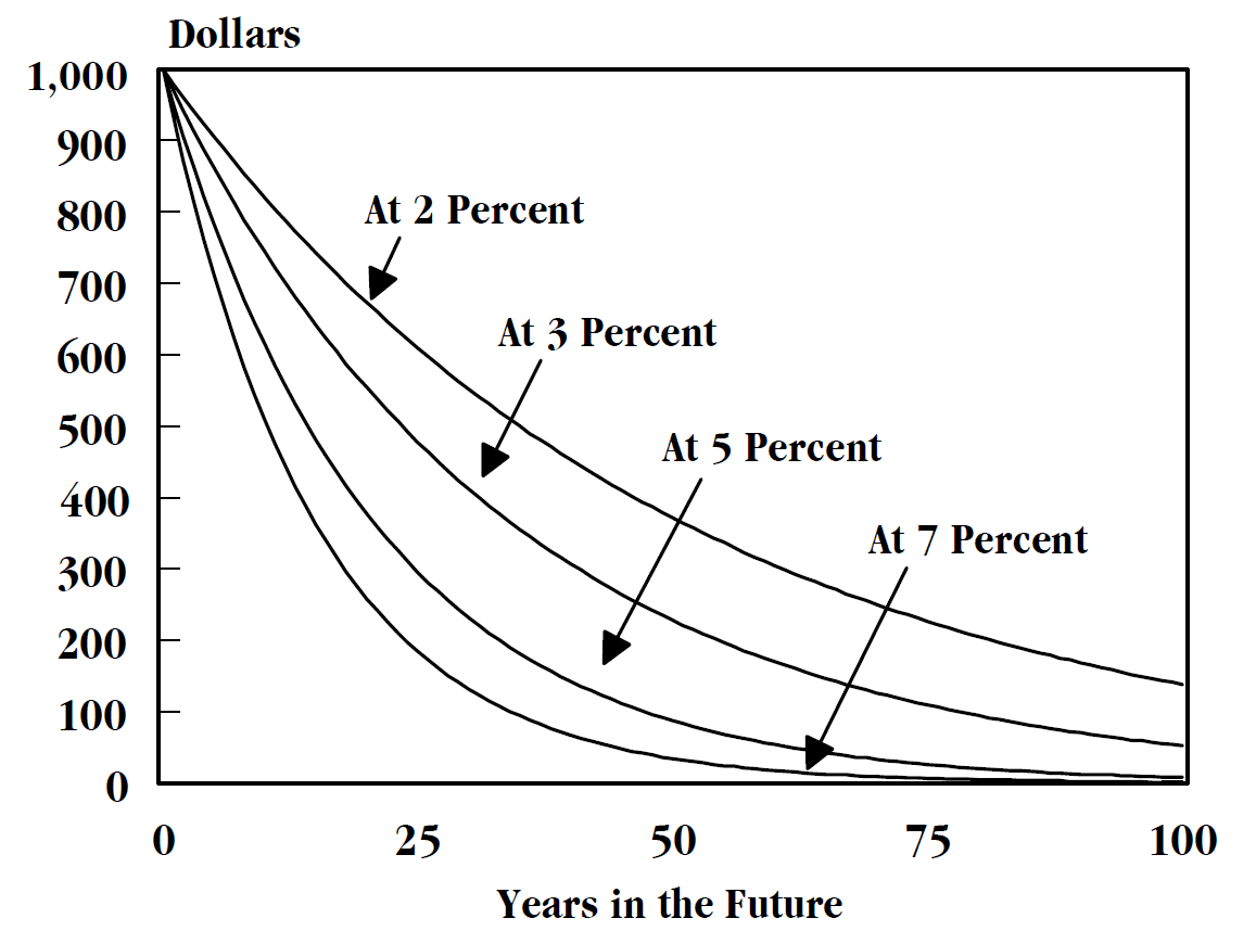
We wish to calculate the present value, also known as the "discounted value" of a payment. Note that a payment made in the future is worth less than the same payment made today which could immediately be deposited into a bank account and earn interest, or invest in other assets. Hence we must discount future payments. Consider a payment F that is to be made t years in the future, we calculate the present value as

Suppose that we wanted to find the present value, denoted PV of $100 that will be received in five years time. If the interest rate r is 12% per year then

Discount rate
[edit]The discount rate which is used in financial calculations is usually chosen to be equal to the cost of capital. The cost of capital, in a financial market equilibrium, will be the same as the market rate of return on the financial asset mixture the firm uses to finance capital investment. Some adjustment may be made to the discount rate to take account of risks associated with uncertain cash flows, with other developments.
The discount rates typically applied to different types of companies show significant differences:
- Start-ups seeking money: 50–100%
- Early start-ups: 40–60%
- Late start-ups: 30–50%
- Mature companies: 10–25%
The higher discount rate for start-ups reflects the various disadvantages they face, compared to established companies:
- Reduced marketability of ownerships because stocks are not traded publicly
- Small number of investors willing to invest
- High risks associated with start-ups
- Overly optimistic forecasts by enthusiastic founders
One method that looks into a correct discount rate is the capital asset pricing model. This model takes into account three variables that make up the discount rate:
- Risk free rate: The percentage of return generated by investing in risk free securities such as government bonds.
- Beta: The measurement of how a company's stock price reacts to a change in the market. A beta higher than 1 means that a change in share price is exaggerated compared to the rest of shares in the same market. A beta less than 1 means that the share is stable and not very responsive to changes in the market. Less than 0 means that a share is moving in the opposite direction from the rest of the shares in the same market.
- Equity market risk premium: The return on investment that investors require above the risk free rate.
- Discount rate = (risk free rate) + beta * (equity market risk premium)
Discount factor
[edit]The discount factor, DF(T), is the factor by which a future cash flow must be multiplied in order to obtain the present value. For a zero-rate (also called spot rate) r, taken from a yield curve, and a time to cash flow T (in years), the discount factor is:

In the case where the only discount rate one has is not a zero-rate (neither taken from a zero-coupon bond nor converted from a swap rate to a zero-rate through bootstrapping) but an annually-compounded rate (for example if the benchmark is a US Treasury bond with annual coupons) and one only has its yield to maturity, one would use an annually-compounded discount factor:

However, when operating in a bank, where the amount the bank can lend (and therefore get interest) is linked to the value of its assets (including accrued interest), traders usually use daily compounding to discount cash flows. Indeed, even if the interest of the bonds it holds (for example) is paid semi-annually, the value of its book of bond will increase daily, thanks to accrued interest being accounted for, and therefore the bank will be able to re-invest these daily accrued interest (by lending additional money or buying more financial products). In that case, the discount factor is then (if the usual money market day count convention for the currency is ACT/360, in case of currencies such as United States dollar, euro, Japanese yen), with r the zero-rate and T the time to cash flow in years:

or, in case the market convention for the currency being discounted is ACT/365 (AUD, CAD, GBP):

Sometimes, for manual calculation, the continuously-compounded hypothesis is a close-enough approximation of the daily-compounding hypothesis, and makes calculation easier (even though its application is limited to instruments such as financial derivatives). In that case, the discount factor is:

Other discounts
[edit]For discounts in marketing, see discounts and allowances, sales promotion, and pricing. The article on discounted cash flow provides an example about discounting and risks in real estate investments.
See also
[edit]References
[edit]Notes
- ^ a b c d e f g h See "Time Value", "Discount", "Discount Yield", "Compound Interest", "Efficient Market", "Market Value" and "Opportunity Cost" in Downes, J. and Goodman, J. E. Dictionary of Finance and Investment Terms, Baron's Financial Guides, 2003.
- ^ a b c d e f g h i j See "Discount", "Compound Interest", "Efficient Markets Hypothesis", "Efficient Resource Allocation", "Pareto-Optimality", "Price", "Price Mechanism" and "Efficient Market" in Black, John, Oxford Dictionary of Economics, Oxford University Press, 2002.
- ^ Chabris, C.F.; Laibson, D.I. & Schuldt, J.P. (2008). "Intertemporal Choice". The New Palgrave Dictionary of Economics.
- ^ Here, the discount rate is different from the discount rate the nation's Central Bank charges financial institutions.
- ^ Kazmi, Kumail (February 26, 2021). "Discount Calculator - Find discounted product price". Smadent.com. Smadent. Retrieved February 26, 2021.
Since a person can earn a return on money
- ^ a b c Competition from other firms who offer other financial assets that promise the market rate of return forces the person who is asking for a delay in payment to offer a "discount yield" that is the same as the market rate of return.
- ^ a b Chiang, Alpha C. (1984). Fundamental Methods of Mathematical Economics (Third ed.). New York: McGraw-Hill. ISBN 0-07-010813-7.
External links
[edit]Discounting
View on GrokipediaFundamentals
Definition and Principles
Discounting is a financial and economic technique used to calculate the present value of future cash flows, benefits, or costs by reducing their nominal amount to reflect the passage of time and associated preferences or risks.[2] This process enables informed decision-making in contexts involving uncertainty, such as investments or policy evaluations, by equating values across different time periods based on the principle that future outcomes are worth less today.[2] At its core, discounting embodies the time value of money, where a dollar today is preferable to a dollar in the future due to potential uses or erosions in value.[6] The origins of discounting trace back to 17th- and 18th-century European finance, where it emerged as a practical tool for valuing long-term obligations amid economic changes like inflation during the "price revolution."[7] In 1626, English clergy at Durham Cathedral applied early discounting tables from published works, such as those in Richard Witt's Arithmeticall Questions (1613), to adjust tenant lease fees for future payments without overburdening lessees during post-Reformation instability.[7] By the 18th century, philosophers like Jeremy Bentham acknowledged the psychological tendency to discount future pleasures or benefits over time within utilitarian thought, though he argued against applying individual time preferences to government policies on consumption and savings.[8] This conceptual foundation was formalized by economist Irving Fisher in his seminal 1930 work, The Theory of Interest, which framed interest and discounting as arising from individual impatience to consume and opportunities for alternative investments.[9] Key principles driving discounting include opportunity cost—the forgone returns from deploying capital elsewhere—and inflation, which erodes the purchasing power of future sums.[10] These factors underscore why present consumption or investment is prioritized over deferred equivalents.[10] Nominal discounting incorporates both the real return and expected inflation into the adjustment, while real discounting isolates the pure time preference by excluding inflationary effects; the relationship is captured by the Fisher equation: where is the nominal rate, is the real rate, and is the inflation rate.[9] Conceptually, discounting thus reflects innate human traits like impatience for immediate rewards and aversion to the uncertainties of future events, without prescribing specific adjustment magnitudes.[9]Time Value of Money
The time value of money (TVM) is the economic principle that a sum of money available today is worth more than the same sum in the future, due to its potential to earn returns, the erosive effects of inflation, and inherent uncertainties. This concept underpins intertemporal decision-making in finance and economics, reflecting how individuals and entities prefer immediate consumption or investment over deferred gratification.[11] The primary drivers of TVM include opportunity cost, inflation, and risk. Opportunity cost arises because money held today can be invested in alternatives like bonds or stocks, generating returns that increase its future value; for instance, forgoing immediate use allows for productive deployment in income-earning assets. Inflation erodes the purchasing power of future money, as rising prices mean a dollar tomorrow buys fewer goods than one today. Risk accounts for the uncertainty of receiving future payments, such as default or economic volatility, which demands compensation in the form of higher expected returns.[11][12] Compounding represents the inverse process to discounting, illustrating TVM by showing how present money grows over time through reinvested earnings. For example, $100 invested today at a positive return rate could expand to substantially more than $100 in the future, as interest accrues on both the principal and prior interest, amplifying wealth accumulation. This growth mechanism highlights why delaying receipt diminishes value unless offset by equivalent earnings potential.[13] A key psychological element in TVM is the pure time preference rate, which captures individuals' inherent impatience in intertemporal choice, valuing present utility more highly than equivalent future utility solely due to its immediacy, independent of economic factors like risk or productivity. This rate influences consumption-saving decisions and interest rates in economic models.[14] The theoretical foundations of TVM trace back to Austrian economists, particularly Eugen von Böhm-Bawerk, whose seminal work Capital and Interest (1884–1909) explained positive interest rates through time preference, arguing that people undervalue future goods relative to present ones due to inherent human impatience, productivity differences in time-intensive production, and variations in foresight across individuals. Böhm-Bawerk's analysis integrated these into a theory of capital as "roundabout" production processes that yield higher returns over time, establishing time preference as central to interest and discounting.[15]Mathematical Components
Discount Rate
The discount rate is the interest rate applied to future cash flows to determine their present value, serving as the required rate of return that investors demand or the cost of capital for a project or investment.[16] It reflects the opportunity cost of capital and compensates for time value, risk, and other factors inherent in delaying consumption or investment.[17] Determining the discount rate typically begins with the risk-free rate, often proxied by yields on long-term government bonds like U.S. Treasuries, which represent returns on theoretically default-free investments.[18] To this base, premiums are added to account for inflation expectations, which erode purchasing power; liquidity risk, which compensates for assets that may be harder to sell quickly without loss; and default risk, which addresses the possibility of non-payment by the issuer or borrower.[19] These components ensure the rate aligns with the investment's specific context, such as nominal versus real terms.[20] A widely adopted method for estimating the discount rate in equity contexts is the Capital Asset Pricing Model (CAPM), formulated as , where denotes the expected return on the asset, is the risk-free rate, measures the asset's systematic risk relative to the market, and is the expected market return.[21] This model, originally developed by William Sharpe, quantifies how non-diversifiable market risk influences the required return beyond the risk-free baseline.[22] Typical discount rates vary by application: long-term social discount rates for public policy evaluations, such as environmental or infrastructure projects, generally range from 3% to 5%, reflecting intergenerational equity considerations.[23] In contrast, corporate equity discount rates, incorporating higher risk premiums, typically span 8% to 12% across industries, as evidenced by sector averages in cost-of-capital datasets.[24] For instance, as of November 2025, the U.S. 10-year Treasury yield stands at approximately 4.11%, providing a current risk-free benchmark amid stable economic conditions.[25] The selection of the discount rate profoundly influences financial outcomes, as even small increases can substantially reduce the present value of distant cash flows, particularly for long-term or high-uncertainty projects where higher rates are warranted to reflect elevated risk.[26] This sensitivity underscores the importance of robust estimation to avoid over- or undervaluing investments.[27]Discount Factor
The discount factor serves as the multiplier applied to a future cash flow to determine its equivalent present value, accounting for the time value of money through the chosen discount rate and the number of periods until receipt. In discrete compounding scenarios, it is calculated using the formula where is the discount rate per period and is the number of periods into the future.[28] This factor decreases exponentially as increases, reflecting the compounding effect that progressively diminishes the present value of cash flows occurring further in the future; for instance, at a 10% discount rate, a cash flow in year 10 is worth only about 38.6% of its nominal amount today.[28] To illustrate, the following table shows discount factors for a 5% annual discount rate over periods 1 to 10, rounded to three decimal places:| Period (t) | Discount Factor |
|---|---|
| 1 | 0.952 |
| 2 | 0.907 |
| 3 | 0.864 |
| 4 | 0.823 |
| 5 | 0.784 |
| 6 | 0.746 |
| 7 | 0.711 |
| 8 | 0.677 |
| 9 | 0.645 |
| 10 | 0.614 |
Core Calculations
Present Value of Single Payments
The present value (PV) of a single future payment represents the current worth of a one-time cash flow expected to occur at a specific future date, discounted back to the present using an appropriate interest rate. This concept stems directly from the compound interest framework, where the future value (FV) of an initial amount invested at a periodic rate over periods is given by . Rearranging this equation to solve for the initial amount yields the core discounting formula: This derivation illustrates that the present value is obtained by dividing the future amount by the compound growth factor over the time horizon, effectively reversing the compounding process to account for the time value of money.[30][31] To apply this formula, consider a step-by-step calculation for a $1,000 payment due in 3 years at an annual discount rate of 7%, assuming annual compounding. First, compute the discount factor for each year: year 1 is ; year 2 is ; year 3 is . Multiply the future value by this cumulative factor: . Alternatively, compute directly: , so . Financial calculators, such as the Texas Instruments BA II Plus, streamline this process: enter N=3 (periods), I/Y=7 (rate), FV=1000 (future value), and compute PV, which yields -816.30 (negative due to sign convention, discussed below).[31][32] In handling negative cash flows, such as loan repayments, sign conventions ensure consistency in calculations. Outflows (e.g., a future payment made by the investor) are typically entered as negative values, while inflows are positive; for instance, the PV of a $1,000 loan repayment in 3 years would be computed as a negative amount, indicating a cost today. This convention aligns cash inflows and outflows in discounted cash flow models, where the net present value is the sum of signed PVs.[32][31] The single-payment PV formula assumes a constant discount rate throughout the period and the absence of any intermediate cash flows, focusing solely on an isolated future amount at a discrete end point. These simplifications hold under deterministic conditions but may require adjustments for varying rates or uncertainty in practice.[31]Present Value of Annuities and Perpetuities
An annuity represents a series of equal payments made at regular intervals over a finite period, and its present value is calculated by discounting each payment back to the present using the discount rate. The present value of an ordinary annuity, where payments occur at the end of each period, is given by the formula: where is the periodic payment amount, is the discount rate per period, and is the number of periods.[33] This formula derives from summing the present values of individual payments, building on the single payment present value as a foundational component.[33] For example, the present value of $100 annual payments for 5 years at a 5% discount rate is approximately $432.95, calculated as .[33] An annuity due, where payments occur at the beginning of each period, has a higher present value due to the earlier timing of cash flows; its formula adjusts the ordinary annuity by multiplying by : This adjustment reflects the one-period advance in payment timing.[33] A perpetuity extends the annuity concept to an infinite number of periods, with the present value simplifying to: assuming constant payments.[34] For a growing perpetuity, where payments increase at a constant rate (with ), the formula becomes: This variant is commonly applied in the dividend discount model to value stocks with perpetually growing dividends; for instance, a stock paying a $2 annual dividend growing at 2% with a 7% required return has a present value of $40.[34]Financial Applications
Discounted Cash Flow Valuation
The discounted cash flow (DCF) valuation model determines the intrinsic value of an asset or project by summing the present values of its expected future free cash flows and subtracting the initial investment outlay. This method assumes that the value of an investment is the discounted sum of all future cash inflows it generates, reflecting the time value of money and opportunity costs. DCF is a cornerstone of financial analysis, applicable to corporate valuations, mergers and acquisitions, and project assessments, where forecasts typically span 5 to 10 years before incorporating a terminal value for perpetuity.[35] In practice, DCF relies on free cash flow to the firm (FCFF) as the primary cash flow metric, which captures the operating cash generated after accounting for taxes, reinvestments, and working capital needs but before financing costs. FCFF is computed as EBIT(1 - tax rate) + depreciation and amortization - capital expenditures - change in net working capital, ensuring the valuation reflects cash available to all capital providers without distortion from leverage. This adjustment isolates the business's core operating performance, making it suitable for discounting at the weighted average cost of capital (WACC).[36] For projections extending beyond the explicit forecast period, a terminal value accounts for the residual worth, commonly estimated via the perpetuity growth model (also known as the Gordon growth model). The formula is: where is the expected cash flow in the first year post-forecast, is the discount rate, and is the long-term growth rate (assumed stable and less than ). This terminal value is then discounted back to the present using the same rate, representing a significant portion—often over 60%—of the total DCF value in mature businesses.[37] To demonstrate the DCF process for a project, consider an initial investment of $8,850 with forecasted free cash flows of $2,000 in year 1, $2,500 in year 2, and $3,000 in years 3 through 5, discounted at 10%. The present value of each cash flow is calculated as follows:- Year 1:
- Year 2:
- Year 3:
- Year 4:
- Year 5: