

Community hub
Recent from talks
Contribute something
Nothing was collected or created yet.
Evolutionary algorithm
View on Wikipedia| Part of a series on the |
| Evolutionary algorithm |
|---|
 |
| Genetic algorithm (GA) |
| Genetic programming (GP) |
| Differential evolution |
| Evolution strategy |
| Evolutionary programming |
| Related topics |
| Part of a series on |
| Artificial intelligence (AI) |
|---|
Evolutionary algorithms (EA) reproduce essential elements of biological evolution in a computer algorithm in order to solve "difficult" problems, at least approximately, for which no exact or satisfactory solution methods are known. They are metaheuristics and population-based bio-inspired algorithms[1] and evolutionary computation, which itself are part of the field of computational intelligence.[2] The mechanisms of biological evolution that an EA mainly imitates are reproduction, mutation, recombination and selection. Candidate solutions to the optimization problem play the role of individuals in a population, and the fitness function determines the quality of the solutions (see also loss function). Evolution of the population then takes place after the repeated application of the above operators.
Evolutionary algorithms often perform well approximating solutions to all types of problems because they ideally do not make any assumption about the underlying fitness landscape. Techniques from evolutionary algorithms applied to the modeling of biological evolution are generally limited to explorations of microevolution (microevolutionary processes) and planning models based upon cellular processes. In most real applications of EAs, computational complexity is a prohibiting factor.[3] In fact, this computational complexity is due to fitness function evaluation. Fitness approximation is one of the solutions to overcome this difficulty. However, seemingly simple EA can solve often complex problems;[4][5][6] therefore, there may be no direct link between algorithm complexity and problem complexity.
Generic definition
[edit]The following is an example of a generic evolutionary algorithm:[7][8][9]
- Randomly generate the initial population of individuals, the first generation.
- Evaluate the fitness of each individual in the population.
- Check, if the goal is reached and the algorithm can be terminated.
- Select individuals as parents, preferably of higher fitness.
- Produce offspring with optional crossover (mimicking reproduction).
- Apply mutation operations on the offspring.
- Select individuals preferably of lower fitness for replacement with new individuals (mimicking natural selection).
- Return to 2
Types
[edit]Similar techniques differ in genetic representation and other implementation details, and the nature of the particular applied problem.
- Genetic algorithm – This is the most popular type of EA. One seeks the solution of a problem in the form of strings of numbers (traditionally binary, although the best representations are usually those that reflect something about the problem being solved),[3] by applying operators such as recombination and mutation (sometimes one, sometimes both). This type of EA is often used in optimization problems.
- Genetic programming – Here the solutions are in the form of computer programs, and their fitness is determined by their ability to solve a computational problem. There are many variants of Genetic Programming:
- Evolutionary programming – Similar to evolution strategy, but with a deterministic selection of all parents.
- Evolution strategy (ES) – Works with vectors of real numbers as representations of solutions, and typically uses self-adaptive mutation rates. The method is mainly used for numerical optimization, although there are also variants for combinatorial tasks.[10][11][12]
- Differential evolution – Based on vector differences and is therefore primarily suited for numerical optimization problems.
- Coevolutionary algorithm – Similar to genetic algorithms and evolution strategies, but the created solutions are compared on the basis of their outcomes from interactions with other solutions. Solutions can either compete or cooperate during the search process. Coevolutionary algorithms are often used in scenarios where the fitness landscape is dynamic, complex, or involves competitive interactions.[13][14]
- Neuroevolution – Similar to genetic programming but the genomes represent artificial neural networks by describing structure and connection weights. The genome encoding can be direct or indirect.
- Learning classifier system – Here the solution is a set of classifiers (rules or conditions). A Michigan-LCS evolves at the level of individual classifiers whereas a Pittsburgh-LCS uses populations of classifier-sets. Initially, classifiers were only binary, but now include real, neural net, or S-expression types. Fitness is typically determined with either a strength or accuracy based reinforcement learning or supervised learning approach.
- Quality–Diversity algorithms – QD algorithms simultaneously aim for high-quality and diverse solutions. Unlike traditional optimization algorithms that solely focus on finding the best solution to a problem, QD algorithms explore a wide variety of solutions across a problem space and keep those that are not just high performing, but also diverse and unique.[15][16][17]
Theoretical background
[edit]The following theoretical principles apply to all or almost all EAs.
No free lunch theorem
[edit]The no free lunch theorem of optimization states that all optimization strategies are equally effective when the set of all optimization problems is considered. Under the same condition, no evolutionary algorithm is fundamentally better than another. This can only be the case if the set of all problems is restricted. This is exactly what is inevitably done in practice. Therefore, to improve an EA, it must exploit problem knowledge in some form (e.g. by choosing a certain mutation strength or a problem-adapted coding). Thus, if two EAs are compared, this constraint is implied. In addition, an EA can use problem specific knowledge by, for example, not randomly generating the entire start population, but creating some individuals through heuristics or other procedures.[18][19] Another possibility to tailor an EA to a given problem domain is to involve suitable heuristics, local search procedures or other problem-related procedures in the process of generating the offspring. This form of extension of an EA is also known as a memetic algorithm. Both extensions play a major role in practical applications, as they can speed up the search process and make it more robust.[18][20]
Convergence
[edit]For EAs in which, in addition to the offspring, at least the best individual of the parent generation is used to form the subsequent generation (so-called elitist EAs), there is a general proof of convergence under the condition that an optimum exists. Without loss of generality, a maximum search is assumed for the proof:
From the property of elitist offspring acceptance and the existence of the optimum it follows that per generation an improvement of the fitness of the respective best individual will occur with a probability . Thus:


I.e., the fitness values represent a monotonically non-decreasing sequence, which is bounded due to the existence of the optimum. From this follows the convergence of the sequence against the optimum.
Since the proof makes no statement about the speed of convergence, it is of little help in practical applications of EAs. But it does justify the recommendation to use elitist EAs. However, when using the usual panmictic population model, elitist EAs tend to converge prematurely more than non-elitist ones.[21] In a panmictic population model, mate selection (see step 4 of the generic definition) is such that every individual in the entire population is eligible as a mate. In non-panmictic populations, selection is suitably restricted, so that the dispersal speed of better individuals is reduced compared to panmictic ones. Thus, the general risk of premature convergence of elitist EAs can be significantly reduced by suitable population models that restrict mate selection.[22][23]
Virtual alphabets
[edit]With the theory of virtual alphabets, David E. Goldberg showed in 1990 that by using a representation with real numbers, an EA that uses classical recombination operators (e.g. uniform or n-point crossover) cannot reach certain areas of the search space, in contrast to a coding with binary numbers.[24] This results in the recommendation for EAs with real representation to use arithmetic operators for recombination (e.g. arithmetic mean or intermediate recombination). With suitable operators, real-valued representations are more effective than binary ones, contrary to earlier opinion.[25][26]
Comparison to other concepts
[edit]Biological processes
[edit]A possible limitation[according to whom?] of many evolutionary algorithms is their lack of a clear genotype–phenotype distinction. In nature, the fertilized egg cell undergoes a complex process known as embryogenesis to become a mature phenotype. This indirect encoding is believed to make the genetic search more robust (i.e. reduce the probability of fatal mutations), and also may improve the evolvability of the organism.[27][28] Such indirect (also known as generative or developmental) encodings also enable evolution to exploit the regularity in the environment.[29] Recent work in the field of artificial embryogeny, or artificial developmental systems, seeks to address these concerns. And gene expression programming successfully explores a genotype–phenotype system, where the genotype consists of linear multigenic chromosomes of fixed length and the phenotype consists of multiple expression trees or computer programs of different sizes and shapes.[30][improper synthesis?]
Monte-Carlo methods
[edit]Both method classes have in common that their individual search steps are determined by chance. The main difference, however, is that EAs, like many other metaheuristics, learn from past search steps and incorporate this experience into the execution of the next search steps in a method-specific form. With EAs, this is done firstly through the fitness-based selection operators for partner choice and the formation of the next generation. And secondly, in the type of search steps: In EA, they start from a current solution and change it or they mix the information of two solutions. In contrast, when dicing out new solutions in Monte-Carlo methods, there is usually no connection to existing solutions.[31][32]
If, on the other hand, the search space of a task is such that there is nothing to learn, Monte-Carlo methods are an appropriate tool, as they do not contain any algorithmic overhead that attempts to draw suitable conclusions from the previous search. An example of such tasks is the proverbial search for a needle in a haystack, e.g. in the form of a flat (hyper)plane with a single narrow peak.
Applications
[edit]The areas in which evolutionary algorithms are practically used are almost unlimited[6] and range from industry,[33][34] engineering,[3][4][35] complex scheduling,[5][36][37] agriculture,[38] robot movement planning[39] and finance[40][41] to research[42][43] and art. The application of an evolutionary algorithm requires some rethinking from the inexperienced user, as the approach to a task using an EA is different from conventional exact methods and this is usually not part of the curriculum of engineers or other disciplines. For example, the fitness calculation must not only formulate the goal but also support the evolutionary search process towards it, e.g. by rewarding improvements that do not yet lead to a better evaluation of the original quality criteria. For example, if peak utilisation of resources such as personnel deployment or energy consumption is to be avoided in a scheduling task, it is not sufficient to assess the maximum utilisation. Rather, the number and duration of exceedances of a still acceptable level should also be recorded in order to reward reductions below the actual maximum peak value.[44] There are therefore some publications that are aimed at the beginner and want to help avoiding beginner's mistakes as well as leading an application project to success.[44][45][46] This includes clarifying the fundamental question of when an EA should be used to solve a problem and when it is better not to.
Related techniques and other global search methods
[edit]There are some other proven and widely used methods of nature inspired global search techniques such as
- Memetic algorithm – A hybrid method, inspired by Richard Dawkins's notion of a meme. It commonly takes the form of a population-based algorithm (frequently an EA) coupled with individual learning procedures capable of performing local refinements. Emphasizes the exploitation of problem-specific knowledge and tries to orchestrate local and global search in a synergistic way.[47]
- A cellular evolutionary or memetic algorithm uses a topological neighborhood relation between the individuals of a population for restricting the mate selection and by that reducing the propagation speed of above-average individuals. The idea is to maintain genotypic diversity in the population over a longer period of time to reduce the risk of premature convergence.[48]
- Ant colony optimization is based on the ideas of ant foraging by pheromone communication to form paths. Primarily suited for combinatorial optimization and graph problems.
- Particle swarm optimization is based on the ideas of animal flocking behaviour. Also primarily suited for numerical optimization problems.
- Gaussian adaptation – Based on information theory. Used for maximization of manufacturing yield, mean fitness or average information. See for instance Entropy in thermodynamics and information theory.[49]
In addition, many new nature-inspired or metaphor-guided algorithms have been proposed since the beginning of this century[when?]. For criticism of most publications on these, see the remarks at the end of the introduction to the article on metaheuristics.
Examples
[edit]In 2020, Google stated that their AutoML-Zero can successfully rediscover classic algorithms such as the concept of neural networks.[50]
The computer simulations Tierra and Avida attempt to model macroevolutionary dynamics.
Gallery
[edit]-
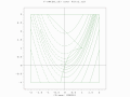 A two-population EA search over a constrained Rosenbrock function with bounded global optimum
 -
 A two-population EA search over a constrained Rosenbrock function. Global optimum is not bounded.
 -

-
 A two-population EA search of a bounded optima of Simionescu's function
.gif)
.gif)

References
[edit]- ^ Farinati, Davide; Vanneschi, Leonardo (December 2024). "A survey on dynamic populations in bio-inspired algorithms". Genetic Programming and Evolvable Machines. 25 (2) 19. doi:10.1007/s10710-024-09492-4. hdl:10362/170138.
- ^ Vikhar, P. A. (2016). "Evolutionary algorithms: A critical review and its future prospects". 2016 International Conference on Global Trends in Signal Processing, Information Computing and Communication (ICGTSPICC). Jalgaon. pp. 261–265. doi:10.1109/ICGTSPICC.2016.7955308. ISBN 978-1-5090-0467-6. S2CID 22100336.
{{cite book}}: CS1 maint: location missing publisher (link) - ^ a b c Cohoon, J. P.; Karro, J.; Lienig, J. (2003). "Evolutionary Algorithms for the Physical Design of VLSI Circuits" in Advances in Evolutionary Computing: Theory and Applications (PDF). London: Springer Verlag. pp. 683–712. ISBN 978-3-540-43330-9.
- ^ a b Slowik, Adam; Kwasnicka, Halina (2020). "Evolutionary algorithms and their applications to engineering problems". Neural Computing and Applications. 32 (16): 12363–12379. doi:10.1007/s00521-020-04832-8. ISSN 0941-0643. S2CID 212732659.
- ^ a b Mika, Marek; Waligóra, Grzegorz; Węglarz, Jan (2011). "Modelling and solving grid resource allocation problem with network resources for workflow applications". Journal of Scheduling. 14 (3): 291–306. doi:10.1007/s10951-009-0158-0. ISSN 1094-6136. S2CID 31859338.
- ^ a b "International Conference on the Applications of Evolutionary Computation". The conference is part of the Evo* series. The conference proceedings are published by Springer. Retrieved 2022-12-23.
- ^ Jansen, Thomas; Weyland, Dennis (7 July 2007). "Analysis of evolutionary algorithms for the longest common subsequence problem". Proceedings of the 9th annual conference on Genetic and evolutionary computation. Association for Computing Machinery. pp. 939–946. doi:10.1145/1276958.1277148. ISBN 978-1-59593-697-4.
- ^ Jin, Yaochu (2003). "Evolutionary Algorithms". Advanced Fuzzy Systems Design and Applications. Studies in Fuzziness and Soft Computing. Vol. 112. Physica-Verlag HD. pp. 49–71. doi:10.1007/978-3-7908-1771-3_2. ISBN 978-3-7908-2520-6.
- ^ Tavares, Jorge; Machado, Penousal; Cardoso, Amílcar; Pereira, Francisco B.; Costa, Ernesto (2004). "On the Evolution of Evolutionary Algorithms". Genetic Programming. Lecture Notes in Computer Science. Vol. 3003. Springer. pp. 389–398. doi:10.1007/978-3-540-24650-3_37. ISBN 978-3-540-21346-8.
- ^ Nissen, Volker; Krause, Matthias (1994), "Constrained Combinatorial Optimization with an Evolution Strategy", in Reusch, Bernd (ed.), Fuzzy Logik, Informatik aktuell, Berlin, Heidelberg: Springer, pp. 33–40, doi:10.1007/978-3-642-79386-8_5, ISBN 978-3-642-79386-8
- ^ Coelho, V. N.; Coelho, I. M.; Souza, M. J. F.; Oliveira, T. A.; Cota, L. P.; Haddad, M. N.; Mladenovic, N.; Silva, R. C. P.; Guimarães, F. G. (2016). "Hybrid Self-Adaptive Evolution Strategies Guided by Neighborhood Structures for Combinatorial Optimization Problems". Evol Comput. 24 (4): 637–666. doi:10.1162/EVCO_a_00187. PMID 27258842. S2CID 13582781.
- ^ Slowik, Adam; Kwasnicka, Halina (1 August 2020). "Evolutionary algorithms and their applications to engineering problems". Neural Computing and Applications. 32 (16): 12363–12379. doi:10.1007/s00521-020-04832-8. ISSN 1433-3058.
- ^ Ma, Xiaoliang; Li, Xiaodong; Zhang, Qingfu; Tang, Ke; Liang, Zhengping; Xie, Weixin; Zhu, Zexuan (2019), "A Survey on Cooperative Co-Evolutionary Algorithms.", IEEE Transactions on Evolutionary Computation, 23 (3): 421–441, Bibcode:2019ITEC...23..421M, doi:10.1109/TEVC.2018.2868770, S2CID 125149900
- ^ Popovici, Elena; Bucci, Anthony; Wiegand, R. Paul; De Jong, Edwin D. (2012). "Coevolutionary Principles". In Rozenberg, Grzegorz; Bäck, Thomas; Kok, Joost N. (eds.). Handbook of Natural Computing. Berlin, Heidelberg: Springer Berlin Heidelberg. pp. 987–1033. doi:10.1007/978-3-540-92910-9_31. ISBN 978-3-540-92910-9.
- ^ Pugh, Justin K.; Soros, Lisa B.; Stanley, Kenneth O. (2016-07-12). "Quality Diversity: A New Frontier for Evolutionary Computation". Frontiers in Robotics and AI. 3. doi:10.3389/frobt.2016.00040. ISSN 2296-9144.
- ^ Lehman, Joel; Stanley, Kenneth O. (2011-07-12). "Evolving a diversity of virtual creatures through novelty search and local competition". Proceedings of the 13th annual conference on Genetic and evolutionary computation. New York, NY, USA: ACM. pp. 211–218. doi:10.1145/2001576.2001606. ISBN 9781450305570. S2CID 17338175.
- ^ Cully, Antoine; Clune, Jeff; Tarapore, Danesh; Mouret, Jean-Baptiste (2015-05-27). "Robots that can adapt like animals". Nature. 521 (7553): 503–507. arXiv:1407.3501. Bibcode:2015Natur.521..503C. doi:10.1038/nature14422. ISSN 0028-0836. PMID 26017452. S2CID 3467239.
- ^ a b Davis, Lawrence (1991). Handbook of genetic algorithms. New York: Van Nostrand Reinhold. ISBN 0-442-00173-8. OCLC 23081440.
- ^ Lienig, Jens; Brandt, Holger (1994), Davidor, Yuval; Schwefel, Hans-Paul; Männer, Reinhard (eds.), "An evolutionary algorithm for the routing of multi-chip modules", Parallel Problem Solving from Nature — PPSN III, vol. 866, Berlin, Heidelberg: Springer, pp. 588–597, doi:10.1007/3-540-58484-6_301, ISBN 978-3-540-58484-1, retrieved 2022-10-18
- ^ Neri, Ferrante; Cotta, Carlos; Moscato, Pablo, eds. (2012). Handbook of Memetic Algorithms. Studies in Computational Intelligence. Vol. 379. Berlin, Heidelberg: Springer Berlin Heidelberg. doi:10.1007/978-3-642-23247-3. ISBN 978-3-642-23246-6.
- ^ Leung, Yee; Gao, Yong; Xu, Zong-Ben (1997). "Degree of population diversity - a perspective on premature convergence in genetic algorithms and its Markov chain analysis". IEEE Transactions on Neural Networks. 8 (5): 1165–1176. doi:10.1109/72.623217. ISSN 1045-9227. PMID 18255718.
- ^ Gorges-Schleuter, Martina (1998), Eiben, Agoston E.; Bäck, Thomas; Schoenauer, Marc; Schwefel, Hans-Paul (eds.), "A comparative study of global and local selection in evolution strategies", Parallel Problem Solving from Nature — PPSN V, Lecture Notes in Computer Science, vol. 1498, Berlin, Heidelberg: Springer Berlin Heidelberg, pp. 367–377, doi:10.1007/bfb0056879, ISBN 978-3-540-65078-2, retrieved 2022-10-21
- ^ Dorronsoro, Bernabe; Alba, Enrique (2008). Cellular Genetic Algorithms. Operations Research/Computer Science Interfaces Series. Vol. 42. Boston, MA: Springer US. doi:10.1007/978-0-387-77610-1. ISBN 978-0-387-77609-5.
- ^ Goldberg, David E. (1990), Schwefel, Hans-Paul; Männer, Reinhard (eds.), "The theory of virtual alphabets", Parallel Problem Solving from Nature, Lecture Notes in Computer Science, vol. 496, Berlin/Heidelberg: Springer-Verlag (published 1991), pp. 13–22, doi:10.1007/bfb0029726, ISBN 978-3-540-54148-6, retrieved 2022-10-22
- ^ Stender, J.; Hillebrand, E.; Kingdon, J. (1994). Genetic algorithms in optimisation, simulation, and modelling. Amsterdam: IOS Press. ISBN 90-5199-180-0. OCLC 47216370.
- ^ Michalewicz, Zbigniew (1996). Genetic Algorithms + Data Structures = Evolution Programs (3rd ed.). Berlin Heidelberg: Springer. ISBN 978-3-662-03315-9. OCLC 851375253.
- ^ G.S. Hornby and J.B. Pollack. "Creating high-level components with a generative representation for body-brain evolution". Artificial Life, 8(3):223–246, 2002.
- ^ Jeff Clune, Benjamin Beckmann, Charles Ofria, and Robert Pennock. "Evolving Coordinated Quadruped Gaits with the HyperNEAT Generative Encoding" Archived 2016-06-03 at the Wayback Machine. Proceedings of the IEEE Congress on Evolutionary Computing Special Section on Evolutionary Robotics, 2009. Trondheim, Norway.
- ^ J. Clune, C. Ofria, and R. T. Pennock, "How a generative encoding fares as problem-regularity decreases", in PPSN (G. Rudolph, T. Jansen, S. M. Lucas, C. Poloni, and N. Beume, eds.), vol. 5199 of Lecture Notes in Computer Science, pp. 358–367, Springer, 2008.
- ^ Ferreira, C., 2001. "Gene Expression Programming: A New Adaptive Algorithm for Solving Problems". Complex Systems, Vol. 13, issue 2: 87–129.
- ^ Schwefel, Hans-Paul (1995). Evolution and Optimum Seeking. Sixth-generation computer technology series. New York: Wiley. p. 109. ISBN 978-0-471-57148-3.
- ^ Fogel, David B.; Bäck, Thomas; Michalewicz, Zbigniew, eds. (2000). Evolutionary Computation 1. Bristol ; Philadelphia: Institute of Physics Publishing. pp. xxx and xxxvii (Glossary). ISBN 978-0-7503-0664-5. OCLC 44807816.
- ^ Sanchez, Ernesto; Squillero, Giovanni; Tonda, Alberto (2012). Industrial Applications of Evolutionary Algorithms. Intelligent Systems Reference Library. Vol. 34. Berlin, Heidelberg: Springer Berlin Heidelberg. doi:10.1007/978-3-642-27467-1. ISBN 978-3-642-27466-4.
- ^ Miettinen, Kaisa; Neittaanmäki, Pekka; Mäkelä, M. M.; Périaux, Jacques, eds. (1999). Evolutionary algorithms in engineering and computer science : recent advances in genetic algorithms, evolution strategies, evolutionary programming, genetic programming, and industrial applications. Chichester: Wiley and Sons. ISBN 0-585-29445-3. OCLC 45728460.
- ^ Gen, Mitsuo; Cheng, Runwei (1999-12-17). Genetic Algorithms and Engineering Optimization. Wiley Series in Engineering Design and Automation. Hoboken, NJ, USA: John Wiley & Sons, Inc. doi:10.1002/9780470172261. ISBN 978-0-470-17226-1.
- ^ Dahal, Keshav P.; Tan, Kay Chen; Cowling, Peter I. (2007). Evolutionary scheduling. Berlin: Springer. doi:10.1007/978-3-540-48584-1. ISBN 978-3-540-48584-1. OCLC 184984689.
- ^ Jakob, Wilfried; Strack, Sylvia; Quinte, Alexander; Bengel, Günther; Stucky, Karl-Uwe; Süß, Wolfgang (2013-04-22). "Fast Rescheduling of Multiple Workflows to Constrained Heterogeneous Resources Using Multi-Criteria Memetic Computing". Algorithms. 6 (2): 245–277. doi:10.3390/a6020245. ISSN 1999-4893.
- ^ Mayer, David G. (2002). Evolutionary Algorithms and Agricultural Systems. Boston, MA: Springer US. doi:10.1007/978-1-4615-1717-7. ISBN 978-1-4613-5693-6.
- ^ Blume, Christian (2000), Cagnoni, Stefano (ed.), "Optimized Collision Free Robot Move Statement Generation by the Evolutionary Software GLEAM", Real-World Applications of Evolutionary Computing, LNCS 1803, vol. 1803, Berlin, Heidelberg: Springer, pp. 330–341, doi:10.1007/3-540-45561-2_32, ISBN 978-3-540-67353-8, retrieved 2022-12-28
- ^ Aranha, Claus; Iba, Hitoshi (2008), Wobcke, Wayne; Zhang, Mengjie (eds.), "Application of a Memetic Algorithm to the Portfolio Optimization Problem", AI 2008: Advances in Artificial Intelligence, Lecture Notes in Computer Science, vol. 5360, Berlin, Heidelberg: Springer Berlin Heidelberg, pp. 512–521, doi:10.1007/978-3-540-89378-3_52, ISBN 978-3-540-89377-6, retrieved 2022-12-23
- ^ Chen, Shu-Heng, ed. (2002). Evolutionary Computation in Economics and Finance. Studies in Fuzziness and Soft Computing. Vol. 100. Heidelberg: Physica-Verlag HD. doi:10.1007/978-3-7908-1784-3. ISBN 978-3-7908-2512-1.
- ^ Lohn, J.D.; Linden, D.S.; Hornby, G.S.; Kraus, W.F. (June 2004). "Evolutionary design of an X-band antenna for NASA's Space Technology 5 mission". IEEE Antennas and Propagation Society Symposium, 2004. Vol. 3. pp. 2313–2316 Vol.3. doi:10.1109/APS.2004.1331834. hdl:2060/20030067398. ISBN 0-7803-8302-8.
- ^ Fogel, Gary; Corne, David (2003). Evolutionary Computation in Bioinformatics. Elsevier. doi:10.1016/b978-1-55860-797-2.x5000-8. ISBN 978-1-55860-797-2.
- ^ a b Jakob, Wilfried (2021), Applying Evolutionary Algorithms Successfully - A Guide Gained from Realworld Applications, KIT Scientific Working Papers, vol. 170, Karlsruhe, FRG: KIT Scientific Publishing, arXiv:2107.11300, doi:10.5445/IR/1000135763, S2CID 236318422, retrieved 2022-12-23
- ^ Whitley, Darrell (2001). "An overview of evolutionary algorithms: practical issues and common pitfalls". Information and Software Technology. 43 (14): 817–831. doi:10.1016/S0950-5849(01)00188-4. S2CID 18637958.
- ^ Eiben, A.E.; Smith, J.E. (2015). "Working with Evolutionary Algorithms". Introduction to Evolutionary Computing. Natural Computing Series (2nd ed.). Berlin, Heidelberg: Springer Berlin Heidelberg. pp. 147–163. doi:10.1007/978-3-662-44874-8. ISBN 978-3-662-44873-1. S2CID 20912932.
- ^ Singh, Avjeet; Kumar, Anoj (2021). "Applications of nature-inspired meta-heuristic algorithms: a survey". International Journal of Advanced Intelligence Paradigms. 20 (3/4) 119026: 388–417. doi:10.1504/IJAIP.2021.119026.
- ^ Nguyen, Phan Trung Hai; Sudholt, Dirk (October 2020). "Memetic algorithms outperform evolutionary algorithms in multimodal optimisation". Artificial Intelligence. 287 103345. doi:10.1016/j.artint.2020.103345.
- ^ Ma, Zhongqiang; Wu, Guohua; Suganthan, Ponnuthurai Nagaratnam; Song, Aijuan; Luo, Qizhang (March 2023). "Performance assessment and exhaustive listing of 500+ nature-inspired metaheuristic algorithms". Swarm and Evolutionary Computation. 77 101248. doi:10.1016/j.swevo.2023.101248.
- ^ Gent, Edd (13 April 2020). "Artificial intelligence is evolving all by itself". Science | AAAS. Archived from the original on 16 April 2020. Retrieved 16 April 2020.
- ^ Simionescu, P.A.; Dozier, G.V.; Wainwright, R.L. (2006). "A Two-Population Evolutionary Algorithm for Constrained Optimization Problems" (PDF). 2006 IEEE International Conference on Evolutionary Computation. Proc 2006 IEEE International Conference on Evolutionary Computation. Vancouver, Canada. pp. 1647–1653. doi:10.1109/CEC.2006.1688506. ISBN 0-7803-9487-9. S2CID 1717817. Retrieved 7 January 2017.
{{cite book}}: CS1 maint: location missing publisher (link) - ^ Simionescu, P.A. (2014). Computer Aided Graphing and Simulation Tools for AutoCAD Users (1st ed.). Boca Raton, FL: CRC Press. ISBN 978-1-4822-5290-3.
Bibliography
[edit]- Ashlock, D. (2006), Evolutionary Computation for Modeling and Optimization, Springer, New York, doi:10.1007/0-387-31909-3 ISBN 0-387-22196-4.
- Bäck, T. (1996), Evolutionary Algorithms in Theory and Practice: Evolution Strategies, Evolutionary Programming, Genetic Algorithms, Oxford Univ. Press, New York, ISBN 978-0-19-509971-3.
- Bäck, T., Fogel, D., Michalewicz, Z. (1999), Evolutionary Computation 1: Basic Algorithms and Operators, CRC Press, Boca Raton, USA, ISBN 978-0-7503-0664-5.
- Bäck, T., Fogel, D., Michalewicz, Z. (2000), Evolutionary Computation 2: Advanced Algorithms and Operators, CRC Press, Boca Raton, USA, doi:10.1201/9781420034349 ISBN 978-0-3678-0637-8.
- Banzhaf, W., Nordin, P., Keller, R., Francone, F. (1998), Genetic Programming - An Introduction, Morgan Kaufmann, San Francisco, ISBN 978-1-55860-510-7.
- Eiben, A.E., Smith, J.E. (2003), Introduction to Evolutionary Computing, Springer, Heidelberg, New York, doi:10.1007/978-3-662-44874-8 ISBN 978-3-662-44873-1.
- Holland, J. H. (1992), Adaptation in Natural and Artificial Systems, MIT Press, Cambridge, MA, ISBN 978-0-262-08213-6.
- Michalewicz, Z.; Fogel, D.B. (2004), How To Solve It: Modern Heuristics. Springer, Berlin, Heidelberg, ISBN 978-3-642-06134-9, doi:10.1007/978-3-662-07807-5.
- Benko, Attila; Dosa, Gyorgy; Tuza, Zsolt (2010). "Bin Packing/Covering with Delivery, solved with the evolution of algorithms". 2010 IEEE Fifth International Conference on Bio-Inspired Computing: Theories and Applications (BIC-TA). pp. 298–302. doi:10.1109/BICTA.2010.5645312. ISBN 978-1-4244-6437-1. S2CID 16875144.
- Price, K., Storn, R.M., Lampinen, J.A., (2005). Differential Evolution: A Practical Approach to Global Optimization, Springer, Berlin, Heidelberg, ISBN 978-3-642-42416-8, doi:10.1007/3-540-31306-0.
- Ingo Rechenberg (1971), Evolutionsstrategie - Optimierung technischer Systeme nach Prinzipien der biologischen Evolution (PhD thesis). Reprinted by Fromman-Holzboog (1973). ISBN 3-7728-1642-8
- Hans-Paul Schwefel (1974), Numerische Optimierung von Computer-Modellen (PhD thesis). Reprinted by Birkhäuser (1977).
- Hans-Paul Schwefel (1995), Evolution and Optimum Seeking. Wiley & Sons, New York. ISBN 0-471-57148-2
- Simon, D. (2013), Evolutionary Optimization Algorithms Archived 2014-03-10 at the Wayback Machine, Wiley & Sons, ISBN 978-0-470-93741-9
- Kruse, Rudolf; Borgelt, Christian; Klawonn, Frank; Moewes, Christian; Steinbrecher, Matthias; Held, Pascal (2013), Computational Intelligence: A Methodological Introduction. Springer, London. ISBN 978-1-4471-5012-1, doi:10.1007/978-1-4471-5013-8.
- Rahman, Rosshairy Abd.; Kendall, Graham; Ramli, Razamin; Jamari, Zainoddin; Ku-Mahamud, Ku Ruhana (2017). "Shrimp Feed Formulation via Evolutionary Algorithm with Power Heuristics for Handling Constraints". Complexity. 2017: 1–12. doi:10.1155/2017/7053710.
External links
[edit]Evolutionary algorithm
View on GrokipediaOverview
Definition and Principles
Evolutionary algorithms (EAs) are a class of population-based metaheuristic optimization techniques inspired by the principles of natural evolution, designed to solve complex optimization problems by iteratively evolving a set of candidate solutions toward improved performance.[2] These algorithms maintain a population of individuals, each representing a potential solution to the problem at hand, and apply operators mimicking biological processes such as reproduction, mutation, recombination, and selection to generate successive generations of solutions.[8] The core objective is to maximize or minimize an objective function, often termed the fitness function, which evaluates the quality of each solution without requiring gradient information or differentiability.[9] At their foundation, EAs operate through a generic iterative process that simulates evolutionary dynamics. The process begins with the initialization of a population of randomly generated candidate solutions, providing an initial diverse set of points in the search space.[2] Each individual is then evaluated based on its fitness, quantifying how well it solves the target problem. Selection follows, where fitter individuals are probabilistically chosen as parents to bias the search toward promising regions. Offspring are generated via recombination (crossover), which combines features from selected parents, and mutation, which introduces random variations to promote exploration. Finally, replacement updates the population, often incorporating strategies like elitism to retain the best solutions, before the loop repeats until a termination criterion—such as a maximum number of generations or satisfactory fitness—is met.[8] This cycle ensures progressive adaptation, with the population evolving over generations. The following pseudocode outlines the basic structure of an EA, as described in foundational literature:Initialize [population](/page/Population) P with random [individuals](/page/Individual)
Evaluate fitness of each [individual](/page/Individual) in P
While termination condition not met:
Select parents from P based on fitness
Recombine pairs of parents to produce [offspring](/page/Offspring)
Mutate [offspring](/page/Offspring)
Evaluate [fitness](/page/Offspring) of [offspring](/page/Offspring)
Replace [individuals](/page/Individual) in P with [offspring](/page/Offspring) (e.g., via [elitism](/page/Elitism))
End
Return best [individual](/page/Individual) or [population](/page/Population)
Initialize [population](/page/Population) P with random [individuals](/page/Individual)
Evaluate fitness of each [individual](/page/Individual) in P
While termination condition not met:
    Select parents from P based on fitness
    Recombine pairs of parents to produce [offspring](/page/Offspring)
    Mutate [offspring](/page/Offspring)
    Evaluate [fitness](/page/Offspring) of [offspring](/page/Offspring)
    Replace [individuals](/page/Individual) in P with [offspring](/page/Offspring) (e.g., via [elitism](/page/Elitism))
End
Return best [individual](/page/Individual) or [population](/page/Population)
Historical Development
The roots of evolutionary algorithms trace back to mid-20th-century cybernetics and early computational models of biological processes. In the 1950s, researchers drew inspiration from cybernetic theories exploring self-organization and adaptation in complex systems. A pivotal influence was John von Neumann's work on self-reproducing automata, initiated in the 1940s and formalized through cellular automata models that demonstrated how computational entities could replicate and potentially evolve, laying conceptual groundwork for algorithmic evolution.[10][11] The 1960s marked the emergence of practical simulations mimicking evolutionary dynamics for optimization and problem-solving. Early efforts included stochastic models of natural selection applied to computational tasks, such as Alex Fraser's 1957 simulations of genetic processes and Hans-Joachim Bremermann's 1962 work on optimization via simulated evolution. These laid the foundation for formal algorithms, with key developments including Ingo Rechenberg's introduction of evolution strategies in 1965 at the Technical University of Berlin, focusing on parameter optimization through mutation and selection in engineering contexts. Concurrently, Lawrence J. Fogel developed evolutionary programming starting in 1960, evolving finite-state machines to solve prediction problems, with foundational experiments documented in 1966. John Holland advanced the genetic algorithm framework in the late 1960s at the University of Michigan, emphasizing schema theory and adaptation, though his comprehensive theoretical exposition appeared later.[12][13][14] The 1970s and 1980s saw the field's maturation through seminal publications and growing academic communities. Holland's 1975 book, Adaptation in Natural and Artificial Systems, provided a rigorous theoretical framework for genetic algorithms, establishing them as tools for adaptive systems. In 1985, the first International Conference on Genetic Algorithms (ICGA) in Pittsburgh fostered collaboration among researchers, highlighting applications in diverse domains. David E. Goldberg's 1989 book, Genetic Algorithms in Search, Optimization, and Machine Learning, popularized the approach, bridging theory and practical implementation for broader adoption.[12][15][16] By the 1990s, evolutionary algorithms gained recognition as a core subfield of computational intelligence, with dedicated journals like Evolutionary Computation launching in 1993 and workshops such as the Parallel Problem Solving from Nature series beginning in 1990. The formation of the Evo* conference series in 1998, encompassing events like EuroGP, further solidified the community's international scope and interdisciplinary impact.[12][17]Core Mechanisms
Population Representation and Initialization
In evolutionary algorithms (EAs), population representation refers to the encoding of candidate solutions as data structures that facilitate the application of genetic operators and fitness evaluation. Common representations include binary strings, which are suitable for discrete optimization problems such as the traveling salesman problem, where each bit encodes a binary decision variable; these are foundational in genetic algorithms (GAs) as introduced by Holland. Real-valued vectors, prevalent in evolution strategies (ES), are preferred for continuous optimization domains like parameter tuning in engineering designs, offering direct mapping to real parameters without discretization errors. Tree structures, used in genetic programming (GP), represent solutions as hierarchical expressions or programs, enabling the evolution of complex computational structures such as symbolic regression models. Permutations encode ordered sequences, ideal for scheduling or routing problems, but require specialized operators to maintain validity. Each method has trade-offs: binary strings provide compact encoding but suffer from Hamming cliffs where adjacent genotypes map to distant phenotypes, while real-valued vectors enhance locality but may introduce bias in mutation scaling.[18] Encoding challenges in representations center on locality and heritability, which influence the algorithm's ability to explore and exploit the search space effectively. Locality measures how small genotypic changes correspond to small phenotypic alterations in fitness; poor locality, as in standard binary encoding, can lead to disruptive mutations that hinder convergence. Heritability assesses the similarity between parent and offspring phenotypes under crossover, ensuring that beneficial traits propagate; representations like trees in GP promote high heritability through subtree exchanges but risk bloat if not controlled. To mitigate binary encoding's locality issues, Gray coding is employed, where consecutive integers differ by only one bit, reducing the Hamming cliff effect.[18] Population initialization generates the starting set of individuals, typically through random or structured methods to ensure diversity. Random uniform sampling draws solutions from a uniform distribution over the search space, providing unbiased coverage but potentially clustering in high-dimensional spaces.[19] Heuristic-based approaches, such as Sobol sequences for low-discrepancy sampling, distribute points more evenly than pure randomness.[20] Importance sampling biases initialization toward promising regions using domain knowledge, though it risks premature convergence if the heuristic is inaccurate.[19] Population size, usually ranging from 50 to 1000 individuals, balances diversity and computational efficiency; smaller sizes (e.g., 50) enable rapid early adaptation on simple landscapes but risk stagnation, while larger sizes (e.g., 500) maintain diversity for rugged multimodal problems at higher cost. Empirical studies on De Jong's test functions showed that sizes around 50-100 optimize performance for unimodal cases, with diversity decaying faster in smaller populations due to genetic drift. These choices in representation and initialization directly impact the efficacy of subsequent selection and reproduction, setting the foundation for effective evolution.Operators: Selection, Crossover, and Mutation
Evolutionary algorithms rely on selection operators to choose individuals from the current population for reproduction, favoring those with higher fitness to guide the search toward improved solutions. The primary goal is to balance exploitation of promising regions and exploration of the search space. Common selection methods include roulette wheel selection, also known as proportional selection, where the probability of selecting an individual is given by , with denoting the fitness of individual and the population size; this method, introduced in foundational work on genetic algorithms, promotes fitter individuals but can suffer from premature convergence if fitness values vary greatly. Tournament selection, a stochastic method where individuals (typically to ) are randomly chosen and the fittest among them is selected, offers controlled selection pressure by adjusting ; larger increases exploitation, as detailed in early analyses of its efficiency. Rank-based selection assigns selection probabilities based on an individual's rank in the sorted fitness list rather than absolute fitness, mitigating issues with scaling; linear ranking, for example, uses , where (1 to 2) controls pressure, providing stable performance across fitness landscapes. Crossover operators combine genetic material from two or more parents to produce offspring, enabling the inheritance of beneficial traits and introducing variability. Single-point crossover, a classic binary operator, selects a random position and swaps the segments after it between parents, preserving large building blocks; it was central to early genetic algorithm designs for discrete problems. Uniform crossover randomly chooses each gene from one of the two parents with equal probability (typically 0.5), promoting greater diversity than single-point but risking disruption of schemata; probabilities between 0.5 and 1.0 are common to tune exploration. For real-valued representations, arithmetic crossover computes offspring as a weighted average, , where is a mixing parameter, suitable for continuous optimization. Blend crossover (BLX-) generates offspring from a uniform distribution within , with and often 0.5, enhancing exploration in real-coded algorithms. Simplex crossover (SPX) uses three parents in a geometric simplex to produce offspring, effective for multimodal problems by preserving volume in the search space. Mutation operators introduce random changes to offspring, maintaining diversity and escaping local optima by simulating genetic variation. In binary encodings, bit-flip mutation inverts each bit with probability , where is the string length, ensuring at least one change per individual on average. For real-valued parameters, Gaussian mutation adds noise from a normal distribution , with standard deviation controlling perturbation size; self-adaptive variants adjust based on fitness progress. Polynomial mutation, common in real-coded genetic algorithms, perturbs each variable by , where follows a polynomial distribution bounded by [0,1] with distribution index (typically 20-100 for fine-tuning), promoting smaller changes near current values while allowing larger jumps. Adaptive mutation rates, which vary dynamically (e.g., increasing if convergence stalls), improve robustness across problems. After generating offspring, replacement strategies determine how the new population is formed from parents and offspring, influencing convergence speed and diversity. Generational replacement fully substitutes the population with offspring, promoting rapid exploration but risking loss of good solutions. Steady-state replacement inserts one or few offspring at a time, replacing the worst or randomly selected individuals, which sustains incremental progress; the GENITOR approach exemplifies this by replacing the least fit. Elitism preserves the top (often 1-5% of population) individuals unchanged, ensuring monotonic improvement in best fitness and accelerating convergence. Parameter tuning for operators is crucial, as rates directly affect balance between exploitation and exploration. Crossover rates typically range from 0.6 to 0.9, with lower values for disruptive operators like uniform crossover to avoid excessive randomization; DeJong's early experiments recommended 0.6 for one/two-point crossover. Mutation rates are usually low, 0.001 to 0.1 per gene or individual, to introduce subtle variations without overwhelming crossover; Grefenstette's settings suggested 0.01 for bit-flip in benchmark functions. Adaptive tuning, such as decreasing mutation as generations progress, often yields better results than fixed values.Algorithm Variants
Genetic Algorithms
Genetic algorithms (GAs) form a foundational subset of evolutionary algorithms, emphasizing binary representations and selection mechanisms inspired by natural genetics. Introduced by John Holland in his 1975 framework, GAs represent candidate solutions as fixed-length binary strings, or chromosomes, where each bit corresponds to a decision variable in the optimization problem.[21] This binary encoding allows for straightforward manipulation through genetic operators, enabling the algorithm to explore discrete search spaces efficiently. The core idea relies on the schema theorem, also known as the building blocks hypothesis, which explains how GAs preferentially propagate short, low-order schemata—subsets of the binary string defined by fixed positions and wildcard symbols (*)—with above-average fitness across generations.[21] The standard GA process begins with the initialization of a population of randomly generated binary strings. Each individual's fitness is evaluated using a problem-specific objective function that quantifies solution quality, with higher values indicating better performance. Selection operators, such as roulette wheel selection or tournament selection, probabilistically choose parents based on relative fitness to form a mating pool. Reproduction occurs primarily through crossover, where operators like two-point crossover exchange segments between two parent chromosomes at randomly selected points to create offspring, preserving potentially beneficial schemata while introducing recombination.[21] Mutation then randomly flips individual bits in the offspring with a low probability (typically 1/L, where L is the chromosome length) to maintain diversity and prevent premature convergence. The expected number of instances of a schema H in the next generation is bounded below by the schema theorem: where is the number of individuals containing schema H at time t, is the average fitness of H, is the population average fitness, and are the crossover and mutation probabilities, is the defining length of H (distance between the outermost fixed positions), L is the chromosome length, and is the order of H (number of fixed positions).[21] This inequality demonstrates how selection amplifies fit schemata, while crossover and mutation terms account for potential disruption. Variants of the canonical binary GA address limitations in representation and convergence. Real-coded GAs replace binary strings with floating-point vectors to handle continuous optimization problems more naturally, avoiding issues like Hamming cliffs in binary encodings where small parameter changes require multiple bit flips. For multimodal problems with multiple optima, niching techniques such as crowding—where similar individuals compete locally—promote the discovery and maintenance of diverse solutions by partitioning the population into subpopulations or niches.[22] These adaptations enhance GA applicability while retaining the core simplicity that makes binary GAs particularly effective for discrete optimization tasks, such as scheduling or feature selection, where the search space is combinatorial.[21]Evolution Strategies and Differential Evolution
Evolution strategies (ES) emerged in the 1960s as a class of evolutionary algorithms tailored for continuous optimization problems, primarily developed by Ingo Rechenberg and Hans-Paul Schwefel at the Technical University of Berlin.[23] Rechenberg's foundational work in his 1973 book introduced ES as a method to optimize technical systems by mimicking biological evolution through iterative mutation and selection on real-valued parameters.[24] Schwefel extended this in his 1977 dissertation, formalizing multi-parent strategies for numerical optimization of computer models.[25] In ES, populations are denoted using (μ, λ) or (μ + λ) schemes, where μ represents the number of parent individuals and λ the number of offspring generated per generation.[25] The (μ/λ)-ES (comma selection) replaces parents solely with offspring, promoting exploration in unbounded search spaces, while the (μ + λ)-ES (plus selection) selects the best μ individuals from the combined pool of μ parents and λ offspring, balancing exploitation and exploration.[26] A key innovation in ES is self-adaptation of mutation parameters, where each individual consists of an object variable vector (the solution parameters) and a strategy parameter vector, typically standard deviations , which evolve alongside through mutation and selection.[24] Mutation in classical ES perturbs object variables using a normal distribution: , where controls the step size for the i-th dimension.[27] Strategy parameters are adapted mutatively, often via multiplicative factors drawn from log-normal distributions to ensure positive values.[25] Rechenberg proposed the 1/5-success rule for non-self-adaptive step-size control in the (1+1)-ES, adjusting based on the success rate of mutations: if approximately 1/5 of offspring improve fitness, is optimal; rates above 1/5 increase by 20%, below decrease it by 20%.[24] This rule derives from theoretical analysis of progress rates on quadratic models, aiming for a success probability near 0.2 to maximize local progress.[28] Differential evolution (DE), introduced by Rainer Storn and Kenneth Price in 1995, is another evolutionary algorithm specialized for global optimization in continuous, multidimensional spaces.[29] Unlike traditional ES, DE relies on vector differences rather than parametric mutations, enabling robust handling of non-separable and noisy functions.[30] The canonical DE/rand/1/bin variant generates a trial vector for a target individual by adding a scaled difference of two randomly selected distinct vectors and to : where indices (NP is population size) are mutually exclusive and distinct from the current index, and F is a real scaling factor typically in [0.5, 1.0].[29] A binomial crossover then combines with to form the final trial vector , where each component if a random number is less than crossover rate CR (in [0,1]) or if j equals a random index, otherwise .[30] Selection replaces with if yields better fitness, ensuring greedy progress.[29] While ES emphasize self-adaptive local search for parameter tuning in engineering contexts, DE excels in global search through its differential perturbation mechanism, which adaptively scales exploration based on population geometry without explicit strategy parameters.[26][29]Other Specialized Types
Genetic programming (GP) represents a specialized form of evolutionary algorithm that evolves computer programs or mathematical expressions using tree-based representations, where nodes denote functions or terminals, enabling the automatic discovery of structured solutions to problems. Introduced by John Koza, GP employs subtree crossover to exchange branches between program trees and ramped half-and-half initialization to generate diverse initial populations with varying depths, promoting exploration of complex program spaces.[31] Evolutionary programming (EP), developed by Lawrence Fogel in the 1960s, focuses on evolving finite-state machines or behavioral models without crossover, relying instead on mutation to alter structures and tournament selection for reproduction, originally applied to prediction tasks in finite domains.[14] Coevolutionary algorithms extend evolutionary computation by evolving multiple interacting populations, such as competitive setups where one population acts as predators and another as prey in host-parasite models, or cooperative frameworks where subpopulations evolve subcomponents that must integrate effectively. Mitchell Potter's 1997 model of cooperative coevolution decomposes complex problems into parallel evolutionary processes, each optimizing a subset while evaluating fitness through collaboration with representatives from other populations.[32] Neuroevolution applies evolutionary algorithms to the evolution of artificial neural networks, optimizing both weights and topologies to solve control or pattern recognition tasks; a prominent example is NeuroEvolution of Augmenting Topologies (NEAT), which starts with minimal networks and incrementally adds complexity through protected innovation numbers to preserve structural diversity during crossover.[33] Learning classifier systems (LCS) integrate evolutionary algorithms with reinforcement learning to evolve sets of condition-action rules for adaptive decision-making in dynamic environments, as formalized by John Holland in 1986. LCS variants include Michigan-style systems, where individual rules evolve within a shared population via credit assignment like the bucket brigade algorithm, and Pittsburgh-style systems, where complete rule sets compete as single individuals, balancing local adaptation with global optimization.[34] Quality-diversity algorithms aim to generate not just high-performing solutions but a diverse archive of behaviors, mapping them onto a discretized behavioral space; MAP-Elites, introduced in the 2010s, maintains an elite per cell in this map, using variation operators to fill unoccupied niches while maximizing performance within each.[35]Theoretical Foundations
No Free Lunch Theorem
The No Free Lunch (NFL) theorem, formally established by Wolpert and Macready in 1997, asserts that for any two distinct search algorithms and , the expected performance of averaged across all possible objective functions equals that of .[36] This equivalence holds under the assumption of no prior domain knowledge, emphasizing that no algorithm can claim universal superiority without specific problem information.[36] The theorem applies to black-box optimization scenarios, where algorithms evaluate objective functions without accessing their internal structure, operating over a finite search space and output space , with a uniform distribution over all possible functions .[36] Performance is typically measured by the off-equilibrium or on-equilibrium success rate in locating optimal points, leading to the core result that any advantage one algorithm holds on certain functions is exactly offset by disadvantages on others.[36] Mathematically, the NFL theorem can be expressed as: where denotes the uniform distribution over all functions , and represents the performance metric (e.g., probability of finding the optimum after evaluations) of algorithm on function .[36] This formulation underscores the theorem's reliance on the exhaustive averaging over an exponentially large function space, rendering blind optimization equivalent to random enumeration in expectation.[36] In the context of evolutionary algorithms (EAs), the NFL theorem implies that no EA variant—whether genetic algorithms, evolution strategies, or others—can outperform others (or even random search) on average over all problems without incorporating domain-specific biases.[36] Effective performance in EAs thus stems from implicit assumptions about problem structure, such as the building-block hypothesis in genetic algorithms, which posits that solutions combine short, high-fitness schema; these biases yield "free lunch" only when aligned with the target problem class but incur penalties elsewhere.[36] Extensions of the NFL theorem include results for time-varying objective functions, where the equivalence persists if the algorithm lacks knowledge of the variation dynamics, maintaining average performance parity across algorithms.[36] Additionally, partial NFL theorems address restricted subclasses of functions or non-uniform priors, allowing certain algorithms to exhibit superior average performance when their design matches the assumed distribution, as explored in subsequent analyses of biased search landscapes.[36]Convergence and Performance Analysis
Convergence analysis in evolutionary algorithms (EAs) focuses on the probabilistic guarantees that these methods will reach a global optimum under specific conditions. For elitist genetic algorithms (GAs), which preserve the best individuals across generations, convergence to a population containing the global optimum occurs almost surely, provided that mutation introduces novelty with positive probability and the search space is finite. This result, derived from Markov chain models, ensures that the algorithm's state space transitions eventually include the optimal solution with probability one, distinguishing elitist variants from non-elitist ones that may fail to converge globally.[37] Runtime analysis examines the expected number of generations or evaluations needed to achieve the optimum on benchmark problems. In evolution strategies (ES), the (1+1)-ES, which maintains a single parent and offspring and selects the fitter, demonstrates an expected runtime of on the sphere function in dimensions, where the mutation step size is adapted via the 1/5-success rule.[38] This linear convergence arises from the algorithm's ability to progressively reduce the distance to the optimum through Gaussian mutations and elitist selection, providing a foundational bound for more complex ES variants. The computational complexity of EAs is typically characterized by time and space requirements tied to key parameters. The time complexity is , where is the number of generations, the population size, and the cost of evaluating an individual's fitness; this reflects the iterative application of selection, crossover, and mutation across the population. Space complexity is , with denoting the length or dimensionality of each individual representation, as the algorithm must store the current population. These bounds highlight the scalability challenges in high-dimensional problems, where evaluation costs often dominate due to expensive fitness functions. To mitigate high evaluation costs, fitness approximation employs surrogate models that predict fitness values without full simulations. Radial basis function (RBF) networks, which interpolate fitness landscapes using localized basis functions centered at evaluated points, serve as effective surrogates in EAs by reducing the number of true evaluations while maintaining search guidance. These models update incrementally as the population evolves, balancing accuracy and efficiency in expensive optimization scenarios. Theoretical analysis of EAs often leverages virtual alphabets to extend binary representations to higher or infinite cardinalities, facilitating proofs for real-coded variants. In this framework, the continuous search space is partitioned into virtual characters—discrete subintervals—that mimic schema processing in binary GAs, enabling convergence arguments via reduced variance in selection and disruption bounds in crossover. This abstraction reveals how high-cardinality encodings preserve building-block assembly, supporting runtime and convergence results across representation types.Comparisons with Other Methods
Biological Evolution Parallels
Evolutionary algorithms (EAs) are fundamentally inspired by the process of natural selection, as articulated in Charles Darwin's theory, where organisms better adapted to their environment—measured by survival and reproductive success—predominate in subsequent generations. In EAs, this parallels the fitness-based selection operator, which probabilistically favors individuals with superior performance evaluations, thereby mimicking differential reproduction and the "survival of the fittest." This mechanism ensures that advantageous traits or solution components are more likely to persist and propagate within the population, driving adaptation toward problem-specific optima. Genetic variation in biological evolution arises primarily through mutation, which introduces random alterations in DNA sequences, and recombination during meiosis, where genetic material from parental chromosomes is exchanged to produce novel combinations in offspring. These processes directly inspire the mutation and crossover operators in EAs: mutation applies small, stochastic changes to an individual's representation to explore nearby solutions, while crossover blends elements from two parent solutions to generate diverse progeny, promoting the combination of beneficial building blocks. Such mappings allow EAs to emulate the creativity of sexual reproduction in generating variability essential for adaptation. Population dynamics in natural evolution involve the maintenance of a diverse gene pool, but phenomena like genetic drift—random fluctuations in allele frequencies due to finite population sizes—can erode variation, especially in small groups. Similarly, in EAs, diversity loss occurs through mechanisms akin to drift, such as selection pressure reducing population variance or bottlenecks from limited population sizes, potentially leading to premature convergence on suboptimal solutions. Population bottlenecks in biology, where a drastic reduction in numbers accelerates drift and fixation of alleles, parallel scenarios in EAs where elite subsets dominate, underscoring the need for diversity-preserving strategies to counteract these effects.[39] Despite these parallels, EAs differ markedly in scale and directionality from biological evolution: they constitute an accelerated, computationally simulated process confined to discrete generations and guided by human-defined fitness landscapes, contrasting with the slow, undirected progression of natural selection over vast timescales influenced by multifaceted environmental pressures. This directed nature enables EAs to solve optimization problems efficiently but lacks the open-ended complexity of true Darwinian evolution. The Baldwin effect illustrates a nuanced interaction where individual learning or plasticity aids survival, indirectly facilitating genetic evolution by allowing time for favorable mutations to arise and spread. In EAs, this is incorporated through hybrid approaches combining global search with local optimization, where "learned" improvements in one generation bias subsequent genetic adaptations. Neutral evolution, theorized by Motoo Kimura, posits that many genetic changes are selectively neutral and fixed via drift rather than selection, maintaining molecular clock-like rates. In EAs, neutral operators expand the neutral network in the genotype-phenotype map, preserving diversity and enabling neutral exploration that supports eventual adaptive shifts without immediate fitness costs.[40][41]Versus Stochastic Optimization Techniques
Evolutionary algorithms (EAs) differ fundamentally from Monte Carlo methods in their approach to global optimization, as Monte Carlo relies on unbiased random sampling across the search space without incorporating historical information from previous evaluations, while EAs use a population of candidate solutions that evolve through mechanisms like selection and variation to exploit correlations and patterns in the problem landscape.[42][43] This guided evolution allows EAs to achieve more efficient convergence; for instance, in optimizing photodetector parameters, the error metric ε95 scales as N^{-0.74} for EAs versus N^{-0.50} for Monte Carlo under equivalent evaluations (N=10,000), demonstrating EAs' superior exploitation of solution dependencies.[42] However, Monte Carlo's simplicity makes it computationally lighter for initial broad exploration, though it lacks the adaptive refinement that EAs provide for multimodal problems.[43] In contrast to simulated annealing (SA), which traverses the search space via a single-solution trajectory guided by a probabilistic acceptance criterion and a cooling schedule to escape local optima, EAs maintain a parallel population of diverse solutions, enabling broader exploration and recombination of promising traits.[44][45] SA often requires fewer function evaluations (typically 10^3–10^4) and converges faster on unimodal landscapes due to its focused perturbation strategy, but it struggles with diversity in highly deceptive environments where EAs excel by preserving multiple trajectories.[45] Empirical comparisons across benchmark problems show EAs yielding higher-quality solutions than SA at the expense of increased computational demands from population management.[44] Particle swarm optimization (PSO) shares EAs' population-based nature but relies on social-inspired velocity updates where particles adjust positions based on personal and global bests, differing from EAs' genetic inheritance through crossover and mutation that promotes discrete recombination.[46] While PSO suits continuous optimization with linear solution times and no need for explicit ranking, EAs like genetic algorithms are more adaptable to discrete and multi-objective problems, handling non-continuous spaces via binary or permutation encodings.[46] PSO's high risk of premature convergence arises from collective momentum toward local optima, whereas EAs mitigate this through diversity-preserving operators, though PSO generally incurs lower overhead per iteration.[46][45] A core distinction lies in EAs' proficiency for discrete and multi-objective scenarios, where their evolutionary operators facilitate handling combinatorial structures and Pareto fronts more naturally than the trajectory-based updates in SA or velocity models in PSO.[46][43] Hybrids such as memetic algorithms address this by integrating local search techniques—similar to SA's neighborhood exploration—directly into the EA framework, applying them selectively to offspring for intensified exploitation without fully abandoning population-level diversity.[47] These memetic variants outperform pure EAs on multimodal benchmarks by accelerating convergence in rugged landscapes, as the local refinements enhance solution quality while leveraging EAs' global search robustness.[47] Overall, EAs offer greater robustness against local optima trapping compared to these stochastic techniques, thanks to their parallel, adaptive populations that balance exploration and exploitation, but this comes at a higher computational intensity, often requiring orders of magnitude more evaluations for large-scale problems.[45] In practice, EAs' parallelizability mitigates this trade-off on modern hardware, making them preferable for complex, non-convex optimizations where pure random or single-path methods falter.[43]Practical Applications
Engineering and Optimization Problems
Evolutionary algorithms have been extensively applied in engineering design problems, particularly for optimizing complex structures where traditional methods struggle with high-dimensional search spaces. A notable example is antenna design, where genetic algorithms were used to evolve an X-band antenna for NASA's Space Technology 5 (ST5) mission in 2006, resulting in a configuration that met performance requirements while minimizing mass and fitting space constraints.[48] This evolved antenna, known as ST5-33-142-7, was successfully launched and demonstrated the efficacy of evolutionary design in aerospace applications by outperforming human-designed alternatives in simulation tests. Similarly, in structural engineering, genetic algorithms have been employed for truss optimization, aiming to minimize weight subject to stress and displacement constraints; for instance, early work applied discrete genetic algorithms to size and topology optimization of truss structures, achieving up to 20-30% weight reductions in benchmark problems like the 10-bar truss. In scheduling domains, evolutionary algorithms address combinatorial challenges in manufacturing and logistics. For job-shop scheduling in flexible manufacturing systems, genetic algorithms have been adapted to minimize makespan by sequencing operations across machines, with hybrid approaches integrating local search to handle machine assignment and operation ordering, yielding solutions within 5-10% of optimal for standard benchmarks like Kacem instances.[49] Vehicle routing problems, including variants of the traveling salesman problem (TSP), benefit from evolutionary methods that evolve route permutations and vehicle loads to reduce total distance and time; a simple genetic algorithm without explicit trip delimiters, combined with local search, has solved capacitated vehicle routing instances with up to 100 customers, achieving near-optimal results faster than exact solvers.[50] Financial engineering leverages evolutionary algorithms for optimization under uncertainty, particularly in portfolio selection and derivative pricing. In portfolio optimization, genetic algorithms search for asset allocations that maximize expected return while controlling risk, often outperforming mean-variance models in non-normal distributions by incorporating cardinality constraints. For option pricing, evolutionary approaches estimate parameters like volatility from market data or approximate prices for complex payoffs; genetic algorithms have been used to solve the Black-Scholes model inversely, recovering implied volatilities with errors under 1% for European calls, handling uncertainty in inputs like dividends and rates more robustly than numerical quadrature.[51] Applications in agriculture and robotics further illustrate the versatility of evolutionary algorithms in resource-constrained environments. In agriculture, genetic algorithms optimize crop yield by allocating resources like water and fertilizers across fields, maximizing total output while respecting soil and climate variability; multi-objective formulations have selected crop varieties and planting schedules to increase yields by 15-25% in simulated scenarios for crops like soybeans.[52] In robotics, particularly swarm systems, evolutionary algorithms evolve path planning strategies to coordinate multiple agents avoiding obstacles, minimizing collision risks and travel time. Multi-objective optimization in engineering often requires balancing conflicting goals, such as cost versus performance, where evolutionary algorithms excel by approximating Pareto fronts. The Non-dominated Sorting Genetic Algorithm II (NSGA-II), introduced in 2002, uses elitist selection and crowding distance to maintain diversity, efficiently handling trade-offs in problems like truss design or scheduling by generating sets of non-dominated solutions that allow decision-makers to select based on preferences. This approach has been widely adopted for its computational efficiency, converging to diverse Pareto-optimal sets in fewer generations than earlier methods, with applications demonstrating improved trade-off surfaces in structural and routing optimizations.Emerging Uses in AI and Machine Learning
Evolutionary algorithms (EAs) have increasingly integrated with neuroevolution techniques to evolve deep neural network architectures, enabling automated design of complex models without manual specification. In neuroevolution, EAs optimize both the topology and weights of neural networks, addressing challenges in reinforcement learning and control tasks. A notable advancement is the Tensorized NeuroEvolution of Augmenting Topologies (TNEAT), which extends the classic NEAT algorithm by incorporating tensor operations for efficient GPU acceleration, achieving up to 10x speedup in evolving convolutional neural networks for image classification tasks compared to traditional NEAT implementations. NEAT has been applied in dynamic environments, such as network attack detection, where NEAT-evolved networks outperform standard machine learning classifiers in identifying anomalies with higher precision and recall rates.[53] In automated machine learning (AutoML), EAs facilitate the discovery of complete ML algorithms from basic primitives, bypassing human-engineered components. Google's AutoML-Zero framework, introduced in 2020, uses a genetic programming-based EA to evolve simple mathematical operations into full ML programs, rediscovering techniques like gradient descent and neural networks on benchmarks such as MNIST, where evolved algorithms achieved 94% accuracy using fewer than 20 instructions.[54] Complementing this, tools like Tree-based Pipeline Optimization Tool (TPOT) employ genetic programming to automate hyperparameter tuning and pipeline construction, optimizing scikit-learn models for classification and regression; in biomedical applications, TPOT has identified pipelines that improve predictive accuracy by 5-15% over default configurations on datasets like those from the UCI repository.[55] Recent extensions of TPOT integrate with large-scale AutoML workflows, enhancing robustness in high-dimensional data scenarios.[56] Dynamic population sizes in EAs have emerged as a key adaptation for non-stationary problems in AI and ML, where environments change over time, such as in online learning or streaming data. A 2024 survey highlights that adaptive population mechanisms, such as growth or shrinkage based on fitness variance, improve convergence in particle swarm optimization and differential evolution variants, with empirical gains of up to 20% in solution quality on dynamic benchmark functions like the moving peaks problem.[57] These techniques are particularly valuable in ML for handling concept drift, enabling EAs to maintain diversity and track shifting optima in real-time applications like adaptive recommender systems. Hybrid quantum-classical EAs, incorporating the Quantum Approximate Optimization Algorithm (QAOA), represent a frontier for solving combinatorial optimization in ML, such as feature selection and graph-based learning. Post-2022 developments include adaptive QAOA variants that dynamically adjust circuit depths using classical EA optimizers, achieving better approximation ratios (e.g., 0.85 on MaxCut instances) than fixed-layer QAOA on noisy intermediate-scale quantum hardware.[58][59] Recent reviews emphasize quantum-inspired EAs that leverage QAOA for hybrid optimization, demonstrating scalability improvements in training quantum neural networks for tasks like quantum machine learning classification. In generative AI, EAs are being applied to evolve prompts and model configurations for large language models (LLMs), automating the crafting of inputs to enhance output quality and diversity. The EvoPrompt framework (2023) uses genetic algorithms to iteratively mutate and select prompts, yielding significant improvements in task performance on benchmarks such as BIG-Bench Hard (BBH).[60] LLM-based genetic algorithms for prompt engineering have shown promise in niche domains, accelerating adaptation by evolving context-aware instructions that boost accuracy in specialized querying by 10-20%.[61]Examples and Implementations
Classic Case Studies
One of the earliest and most influential applications of evolutionary algorithms in engineering was the automated design of antennas for NASA's Space Technology 5 (ST5) mission in 2006. Researchers at NASA Ames Research Center employed a genetic algorithm to evolve wire antenna geometries, optimizing for radiation patterns, gain, and impedance within strict mission constraints, such as fitting within a 15.24 cm diameter cylinder and a mass limit of under 165 grams. The resulting evolved monopole antenna, known as ST5-33-142-7, achieved 93% efficiency when using two units, compared to 38% for the conventional quadrifilar helix design, while providing higher gain across a wider range of elevation angles to improve data throughput during the spacecraft's low Earth orbit. This compact design not only met the mission's size and power requirements but also reduced design time to approximately three person-months, versus five for traditional methods, and was successfully launched on March 22, 2006, marking the first instance of computer-evolved hardware deployed in space.[62] In function optimization, the (1+1)-evolution strategy (ES), a foundational variant of evolutionary algorithms, demonstrated robust performance on classic benchmark problems like the sphere and Rastrigin functions. Introduced by Ingo Rechenberg in 1973, the (1+1)-ES maintains a single parent solution and generates one offspring through mutation, selecting the fitter individual for the next generation, with self-adaptive step-size control via the 1/5-success rule to balance exploration and exploitation. On the unimodal sphere function, which measures quadratic error from the global optimum, the algorithm exhibits linear convergence in expectation, achieving a progress rate proportional to the standardized step size under optimal adaptation, making it efficient for smooth, separable landscapes. For the multimodal Rastrigin function, featuring numerous local optima due to sinusoidal perturbations, the (1+1)-ES still navigates toward the global minimum through sustained mutation pressure, though at a slower rate than on the sphere, highlighting its resilience in deceptive search spaces as analyzed in early theoretical work. These benchmarks underscored the strategy's practical utility in numerical optimization tasks from the 1970s onward.[26] The Tierra system, developed by Thomas Ray in 1991, provided a pioneering case study in digital evolution by simulating self-replicating computer programs that evolved increasing code complexity in a virtual machine environment. Programs, or "digital organisms," competed for CPU time and memory on a parallel processor, undergoing mutation and natural selection to replicate and execute instructions, leading to the emergence of parasites, hosts, and symbiotic ecologies without explicit fitness functions beyond replication efficiency. Over runs lasting weeks, Tierra organisms evolved from simple replicators to more complex forms with over 80 instructions, demonstrating open-ended evolution and ecological dynamics akin to biological systems, such as the rise of "lattice" organisms that exploited replication shortcuts. This work laid the groundwork for subsequent platforms like Avida, an extension developed in the mid-1990s, which further enabled controlled experiments on evolutionary innovation, including the evolution of complex traits like logic operations through cumulative selection in digital lineages.[63] Evolutionary programming also proved effective in game artificial intelligence, as exemplified by David Fogel's Blondie24 program for checkers in the late 1990s and early 2000s. Using a population-based evolutionary algorithm, Blondie24 evolved finite-state machines to evaluate board positions via artificial neural networks, starting from random strategies and refining them over thousands of self-play games without incorporating human knowledge or opening books. After 800 hours of evolution on a personal computer, Blondie24 achieved an expert-level rating, securing a position in the top 500 of an international online checkers server and defeating commercial programs like Chinook in non-expert matches. This success illustrated how evolutionary methods could autonomously discover competitive strategies through variation and selection, as detailed in Fogel's 2002 analysis, emphasizing the algorithm's ability to generalize across game states. In the realm of art and design, Karl Sims' 1994 work on evolving virtual creatures showcased evolutionary algorithms' creative potential by generating diverse morphologies and behaviors in simulated 3D environments. Genetic algorithms operated on directed graphs encoding creature bodies—composed of rigid segments connected by joints—and neural networks controlling muscle forces, with fitness based on tasks like locomotion speed or obstacle avoidance in physically realistic worlds powered by inverse kinematics and dynamics simulation. Over 50-100 generations with populations of 300 individuals, the system produced creatures exhibiting innovative gaits, such as quadrupedal walking, serpentine swimming, and jumping, often converging on solutions more varied and efficient than hand-designed ones, with evolutions completing in about three hours on a 32-processor supercomputer. Sims' approach highlighted how selection pressures could automate the co-evolution of form and function, influencing later applications in generative art and animation.[64]Modern Computational Examples
In the AutoML-Zero experiment conducted by Google researchers in 2020, evolutionary algorithms were used to discover complete machine learning pipelines from a set of 77 primitive mathematical operations, such as addition, multiplication, and matrix transposition, without relying on pre-defined high-level components like neural network layers.[54] The framework evolves programs consisting of setup, predict, and learn functions, starting from empty programs and iteratively improving them through mutation and crossover on tasks like binary classification of projected CIFAR-10 images.[54] Notable evolved components included weight update mechanisms, such as normalized gradients (where gradients are divided by their L2 norm before application, improving accuracy by 1.20% when ablated) and multiplicative weight perturbations (adding noise scaled by input magnitude, contributing 0.16% to performance).[54] On binary CIFAR-10, the best evolved algorithm achieved 84.06% accuracy, outperforming a hand-designed two-layer neural network baseline of 82.22% when constrained to similar compute budgets, demonstrating the potential to rediscover backpropagation-like techniques autonomously.[54] Dynamic evolutionary algorithms address changing environments, such as those with drifting optima, by adaptively resizing the population size μ to balance exploration and exploitation.[65] A 2024 survey by Farinati and Vanneschi highlights fitness-based strategies, where population adjustments trigger on stagnation or improvement signals; for instance, in dynamic phases with shifting optima, random immigrants are added to inject diversity, while static phases prune underperformers.[65] One representative approach from the survey adapts μ as follows (pseudocode inspired by fitness stagnation detection in referenced works):if fitness_stagnation > threshold: # Static phase detected
select_worst = sort(population, key=fitness)[-n:] # n = μ / 2 worst individuals
remove = select_worst[-μ//2:] # Remove largest among worst
population = population - remove
else: # Dynamic phase, add immigrants
immigrants = generate_random(μ//2)
population += immigrants
μ = len(population)
if fitness_stagnation > threshold:  # Static phase detected
    select_worst = sort(population, key=fitness)[-n:]  # n = μ / 2 worst individuals
    remove = select_worst[-μ//2:]  # Remove largest among worst
    population = population - remove
else:  # Dynamic phase, add immigrants
    immigrants = generate_random(μ//2)
    population += immigrants
    μ = len(population)
import random
from deap import base, creator, tools

# Item weights and values (example: 100 items)
items = [(random.randint(1,10), random.uniform(0,100)) for _ in range(100)]
MAX_WEIGHT = 50
creator.create("FitnessMulti", base.Fitness, weights=(-1.0, 1.0))  # Minimize [weight](/page/The_Weight), maximize value
creator.create("[Individual](/page/Individual)", set, fitness=creator.FitnessMulti)

def evalKnapsack([individual](/page/Individual)):
    [weight](/page/The_Weight), value = 0, 0
    for item in [individual](/page/Individual):
        [weight](/page/The_Weight) += items[item][0]
        value += items[item][1]
    if [weight](/page/The_Weight) > MAX_WEIGHT:
        return 10000, 0  # Penalty
    return [weight](/page/The_Weight), value

toolbox = base.Toolbox()
toolbox.register("individual", tools.initIterate, creator.Individual, lambda: random.sample(range(len(items)), random.randint(1, len(items))))
toolbox.register("population", tools.initRepeat, list, toolbox.individual)
toolbox.register("evaluate", evalKnapsack)
toolbox.register("mate", tools.cxSet)
toolbox.register("mutate", tools.mutSet, weight_func=lambda x: 1/x)  # Higher probability for smaller sets
toolbox.register("select", tools.selNSGA2)

pop = toolbox.population(n=50)
algorithms.eaMuPlusLambda(pop, toolbox, mu=50, lambda_=100, cxpb=0.7, mutpb=0.2, ngen=50, verbose=False)
def crossover(parent1, parent2):  # Assume parent1 more fit
    child_genes = []
    i1, i2 = 0, 0
    while i1 < len(parent1.genes) and i2 < len(parent2.genes):
        if parent1.genes[i1].innovation == parent2.genes[i2].innovation:
            # Matching gene: randomly inherit from either
            child_genes.append(random.choice([parent1.genes[i1], parent2.genes[i2]]))
            i1 += 1; i2 += 1
        elif parent1.genes[i1].innovation < parent2.genes[i2].innovation:
            # Disjoint from parent2: inherit from parent1
            child_genes.append(parent1.genes[i1])
            i1 += 1
        else:
            # Disjoint from parent1: skip (inherit from fitter parent1 later)
            i2 += 1
    # Append excess genes from fitter parent1
    child_genes += parent1.genes[i1:]
    return Genome(child_genes)