
Community hub
Recent from talks
Contribute something
Nothing was collected or created yet.
Image rectification
View on Wikipedia
Image rectification is a transformation process used to project images onto a common image plane. This process has several degrees of freedom and there are many strategies for transforming images to the common plane. Image rectification is used in computer stereo vision to simplify the problem of finding matching points between images (i.e. the correspondence problem), and in geographic information systems (GIS) to merge images taken from multiple perspectives into a common map coordinate system.
In computer vision
[edit]


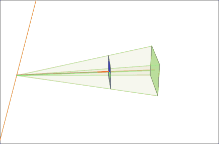
Computer stereo vision takes two or more images with known relative camera positions that show an object from different viewpoints. For each pixel it then determines the corresponding scene point's depth (i.e. distance from the camera) by first finding matching pixels (i.e. pixels showing the same scene point) in the other image(s) and then applying triangulation to the found matches to determine their depth. Finding matches in stereo vision is restricted by epipolar geometry: Each pixel's match in another image can only be found on a line called the epipolar line. If two images are coplanar, i.e. they were taken such that the right camera is only offset horizontally compared to the left camera (not being moved towards the object or rotated), then each pixel's epipolar line is horizontal and at the same vertical position as that pixel. However, in general settings (the camera does move towards the object or rotate) the epipolar lines are slanted. Image rectification warps both images such that they appear as if they have been taken with only a horizontal displacement and as a consequence all epipolar lines are horizontal, which slightly simplifies the stereo matching process. Note however, that rectification does not fundamentally change the stereo matching process: It searches on lines, slanted ones before and horizontal ones after rectification.
Image rectification is also an equivalent (and more often used[1]) alternative to perfect camera coplanarity. Even with high-precision equipment, image rectification is usually performed because it may be impractical to maintain perfect coplanarity between cameras.
Image rectification can only be performed with two images at a time and simultaneous rectification of more than two images is generally impossible.[2]
Transformation
[edit]If the images to be rectified are taken from camera pairs without geometric distortion, this calculation can easily be made with a linear transformation. X & Y rotation puts the images on the same plane, scaling makes the image frames be the same size and Z rotation & skew adjustments make the image pixel rows directly line up[citation needed]. The rigid alignment of the cameras needs to be known (by calibration) and the calibration coefficients are used by the transform.[3]
In performing the transform, if the cameras themselves are calibrated for internal parameters, an essential matrix provides the relationship between the cameras. The more general case (without camera calibration) is represented by the fundamental matrix. If the fundamental matrix is not known, it is necessary to find preliminary point correspondences between stereo images to facilitate its extraction.[3]
Algorithms
[edit]There are three main categories for image rectification algorithms: planar rectification,[4] cylindrical rectification[1] and polar rectification.[5][6][7]
Implementation details
[edit]All rectified images satisfy the following two properties:[8]
- All epipolar lines are parallel to the horizontal axis.
- Corresponding points have identical vertical coordinates.
In order to transform the original image pair into a rectified image pair, it is necessary to find a projective transformation H. Constraints are placed on H to satisfy the two properties above. For example, constraining the epipolar lines to be parallel with the horizontal axis means that epipoles must be mapped to the infinite point [1,0,0]T in homogeneous coordinates. Even with these constraints, H still has four degrees of freedom.[9] It is also necessary to find a matching H' to rectify the second image of an image pair. Poor choices of H and H' can result in rectified images that are dramatically changed in scale or severely distorted.
There are many different strategies for choosing a projective transform H for each image from all possible solutions. One advanced method is minimizing the disparity or least-square difference of corresponding points on the horizontal axis of the rectified image pair.[9] Another method is separating H into a specialized projective transform, similarity transform, and shearing transform to minimize image distortion.[8] One simple method is to rotate both images to look perpendicular to the line joining their collective optical centers, twist the optical axes so the horizontal axis of each image points in the direction of the other image's optical center, and finally scale the smaller image to match for line-to-line correspondence.[2] This process is demonstrated in the following example.
Example
[edit]


Our model for this example is based on a pair of images that observe a 3D point P, which corresponds to p and p' in the pixel coordinates of each image. O and O' represent the optical centers of each camera, with known camera matrices and (we assume the world origin is at the first camera). We will briefly outline and depict the results for a simple approach to find a H and H' projective transformation that rectify the image pair from the example scene.
![{\displaystyle M=K[I~0]}](https://wikimedia.org/api/rest_v1/media/math/render/svg/36bab3ec4fb0bb080e213c2ed255b77a3783af3b)
![{\displaystyle M'=K'[R~T]}](https://wikimedia.org/api/rest_v1/media/math/render/svg/6b49a26dca801d091e45d483e46eb0a17a883c28)
First, we compute the epipoles, e and e' in each image:
![{\displaystyle e=M{\begin{bmatrix}O'\\1\end{bmatrix}}=M{\begin{bmatrix}-R^{T}T\\1\end{bmatrix}}=K[I~0]{\begin{bmatrix}-R^{T}T\\1\end{bmatrix}}=-KR^{T}T}](https://wikimedia.org/api/rest_v1/media/math/render/svg/27b3eb1954bb32452aaee6d928968474f9e3b358)
![{\displaystyle e'=M'{\begin{bmatrix}O\\1\end{bmatrix}}=M'{\begin{bmatrix}0\\1\end{bmatrix}}=K'[R~T]{\begin{bmatrix}0\\1\end{bmatrix}}=K'T}](https://wikimedia.org/api/rest_v1/media/math/render/svg/c2f0d667c156022e71390855e68b60621c65cead)
Second, we find a projective transformation H1 that rotates our first image to be parallel to the baseline connecting O and O' (row 2, column 1 of 2D image set). This rotation can be found by using the cross product between the original and the desired optical axes.[2] Next, we find the projective transformation H2 that takes the rotated image and twists it so that the horizontal axis aligns with the baseline. If calculated correctly, this second transformation should map the e to infinity on the x axis (row 3, column 1 of 2D image set). Finally, define as the projective transformation for rectifying the first image.

Third, through an equivalent operation, we can find H' to rectify the second image (column 2 of 2D image set). Note that H'1 should rotate the second image's optical axis to be parallel with the transformed optical axis of the first image. One strategy is to pick a plane parallel to the line where the two original optical axes intersect to minimize distortion from the reprojection process.[10] In this example, we simply define H' using the rotation matrix R and initial projective transformation H as .

Finally, we scale both images to the same approximate resolution and align the now horizontal epipoles for easier horizontal scanning for correspondences (row 4 of 2D image set).
Note that it is possible to perform this and similar algorithms without having the camera parameter matrices M and M' . All that is required is a set of seven or more image to image correspondences to compute the fundamental matrices and epipoles.[9]
In geographic information system
[edit]Image rectification in GIS converts images to a standard map coordinate system. This is done by matching ground control points (GCP) in the mapping system to points in the image. These GCPs calculate necessary image transforms.[11]
Primary difficulties in the process occur
- when the accuracy of the map points are not well known
- when the images lack clearly identifiable points to correspond to the maps.
The maps that are used with rectified images are non-topographical. However, the images to be used may contain distortion from terrain. Image orthorectification additionally removes these effects.[11]
Image rectification is a standard feature available with GIS software packages.
See also
[edit]References
[edit]- ^ a b Oram, Daniel (2001). Rectification for Any Epipolar Geometry.
- ^ a b c Szeliski, Richard (2010). Computer vision: Algorithms and applications. Springer. ISBN 9781848829350.
- ^ a b Fusiello, Andrea (2000-03-17). "Epipolar Rectification". Archived from the original on 2015-11-13. Retrieved 2008-06-09.
- ^ Fusiello, Andrea; Trucco, Emanuele; Verri, Alessandro (2000-03-02). "A compact algorithm for rectification of stereo pairs" (PDF). Machine Vision and Applications. 12: 16–22. doi:10.1007/s001380050120. S2CID 13250851. Archived from the original (PDF) on 2015-09-23. Retrieved 2010-06-08.
- ^ Pollefeys, Marc; Koch, Reinhard; Van Gool, Luc (1999). "A simple and efficient rectification method for general motion" (PDF). Proc. International Conference on Computer Vision: 496–501. Retrieved 2011-01-19.
- ^ Lim, Ser-Nam; Mittal, Anurag; Davis, Larry; Paragios, Nikos. "Uncalibrated stereo rectification for automatic 3D surveillance" (PDF). International Conference on Image Processing. 2: 1357. Archived from the original (PDF) on 2010-08-21. Retrieved 2010-06-08.
- ^ Roberto, Rafael; Teichrieb, Veronica; Kelner, Judith (2009). "Retificação Cilíndrica: um método eficente para retificar um par de imagens" (PDF). Workshops of Sibgrapi 2009 - Undergraduate Works (in Portuguese). Archived from the original (PDF) on 2011-07-06. Retrieved 2011-03-05.
- ^ a b Loop, Charles; Zhang, Zhengyou (1999). "Computing rectifying homographies for stereo vision" (PDF). Proceedings. 1999 IEEE Computer Society Conference on Computer Vision and Pattern Recognition (Cat. No PR00149). pp. 125–131. CiteSeerX 10.1.1.34.6182. doi:10.1109/CVPR.1999.786928. ISBN 978-0-7695-0149-9. S2CID 157172. Retrieved 2014-11-09.
- ^ a b c Hartley, Richard; Zisserman, Andrew (2003). Multiple view geometry in computer vision. Cambridge university press. ISBN 9780521540513.
- ^ Forsyth, David A.; Ponce, Jean (2002). Computer vision: a modern approach. Prentice Hall Professional Technical Reference.
- ^ a b Fogel, David. "Image Rectification with Radial Basis Functions". Archived from the original on 2008-05-24. Retrieved 2008-06-09.
- Hartley, R. I. (1999). "Theory and Practice of Projective Rectification". International Journal of Computer Vision. 35 (2): 115–127. doi:10.1023/A:1008115206617. S2CID 406463.
- Pollefeys, Marc. "Polar rectification". Retrieved 2007-06-09.[permanent dead link]
- Shapiro, Linda G.; Stockman, George C. (2001). Computer Vision. Prentice Hall. pp. 580. ISBN 978-0-13-030796-5.
Further reading
[edit]- Computing Rectifying Homographies for Stereo Vision by Charles Loop and Zhengyou Zhang (April 8, 1999) Microsoft Research
- Computer Vision: Algorithms and Applications, Section 11.1.1 "Rectification" by Richard Szeliski (September 3, 2010) Springerdheerajnkumar
Image rectification
View on GrokipediaFundamentals
Definition and Purpose
Image rectification is a geometric transformation process in computer vision that applies homographies to a pair of images from different viewpoints, aligning their epipolar lines parallel to a common baseline so that corresponding points share the same row coordinates.[1] This projects the images onto a common fronto-parallel plane, simplifying the search for pixel correspondences by restricting matches to horizontal scanlines and facilitating stereo matching and disparity estimation.[7] In essence, it transforms perspective views to constrain epipolar geometry, enabling efficient depth computation while preserving relative scene structure. The primary purpose of image rectification is to support accurate 3D reconstruction and depth estimation from stereo pairs in computer vision applications, such as robotics and autonomous navigation. By aligning epipolar lines, it reduces the computational complexity of disparity estimation from 2D searches to 1D along rows, improving matching robustness and accuracy.[8] Rectification evolved from foundations in projective geometry, with key developments in epipolar constraint methods advancing digital implementations in computer vision since the late 20th century. Rectification primarily employs projective transformations via homographies to correct perspective distortions and align vanishing points with parallel lines, essential for stereo vision setups.[9] Key distortion sources in unrectified stereo images include perspective effects from camera viewpoints, leading to non-horizontal epipolar lines and scale variations.[10]Mathematical Principles
Image rectification relies on the transformation between different coordinate systems to map points from the real world to the image plane. In the world coordinate system, points are represented in metric units (e.g., meters) as 3D vectors . These are transformed to the camera coordinate system, a 3D frame centered at the camera's optical center with the Z-axis aligned along the optical axis, using extrinsic parameters: a 3x3 rotation matrix and a 3x1 translation vector , such that .[11] The camera coordinate system points are then projected onto the 2D image plane using intrinsic parameters, captured in the 3x3 camera matrix , where and are focal lengths in pixels along the x and y axes, and is the principal point (typically the image center). The projection follows the pinhole model: for a point in camera coordinates, the image coordinates are , or in homogeneous form, . Image coordinates are pixel-based, differing from metric world coordinates by incorporating these intrinsics and extrinsics, which are essential for rectification to align distorted or perspective views with a canonical plane.[11] For planar rectification, a 3x3 homography matrix models the projective transformation between two images of a plane, mapping a point in one image to in the other, up to scale. This arises from the projection of a world plane (defined by , with normal and distance ) through two cameras with projection matrices and , yielding , where and are relative extrinsics and are intrinsics. To estimate without known parameters, the direct linear transformation (DLT) uses at least four point correspondences . Each pair yields two equations from , forming a system where (9 elements, with scale freedom), solved via SVD of (2n × 9 for n points) to find the right singular vector corresponding to the smallest singular value, then reshaping to . This enforces the projective mapping for rectification of planar scenes, such as document scanning.[12] In stereo rectification for non-planar scenes, the fundamental matrix (3x3, rank 2) encodes the epipolar geometry between two views, satisfying for corresponding points , where with relative rotation and translation (normalized such that ). has seven degrees of freedom and can be estimated from at least seven correspondences using similar linear methods, followed by enforcement of rank 2 via SVD. For rectification, decomposes into and : first compute the essential matrix (up to scale), then SVD yields and from the third column of (or similar choices for positive depth), providing the relative pose to align epipolar lines.[13] Lens distortions must be corrected before rectification, as they deviate from the ideal pinhole model. The standard radial distortion model, often up to fourth order, maps undistorted coordinates (relative to distortion center ) to distorted ones via radial distance , with where are coefficients (positive for barrel distortion, negative for pincushion). Tangential distortion, due to lens-sensor misalignment, adds terms with parameters . Correction inverts these: starting from observed distorted pixels, solve iteratively for undistorted coordinates (e.g., via fixed-point iteration or lookup tables), then apply the pinhole projection. These models, estimated during calibration, ensure accurate rectification by removing non-linear warping.[14] Rectification equations for single images use projective transformations to remove perspective distortion, often via homography to map to a frontal view: select control points or lines (e.g., vanishing lines) to solve for such that parallel world lines become parallel in the rectified image, as in where enforces affinity at infinity. For stereo pairs, rectification applies homographies derived from to align epipolar lines horizontally: decompose to find rotation matrices such that new projections and (with shared intrinsics) make the baseline horizontal, yielding where epipoles lie on the x-axis and lines are scanlines . This simplifies disparity computation along rows.[9][15]Computer Vision Applications
Geometric Transformations
The transformation pipeline for image rectification in computer vision typically begins with feature detection to identify salient points in the images, such as Scale-Invariant Feature Transform (SIFT) keypoints, which are robust to scale, rotation, and illumination changes.[16] These features enable correspondence matching between image pairs, often using descriptor similarity metrics like Euclidean distance on SIFT vectors to establish point-to-point associations.[16] Once correspondences are obtained, homography estimation computes a 3x3 transformation matrix that maps points from one image to the other, typically via least-squares optimization on the fundamental matrix or direct linear transformation for planar scenes. The final step involves warping the images using inverse mapping, where for each pixel in the output image, the corresponding source coordinates are computed via , and interpolation (e.g., bilinear) fills values to prevent holes or aliasing. In stereo rectification, the process computes rectification matrices and for calibrated camera pairs to align epipolar lines horizontally, simplifying disparity computation. For calibrated systems with known intrinsics , the new projection matrices are derived as and , where and are rotations that align the optical axes parallel while preserving the baseline, computed by orthogonalizing the relative pose to ensure the translation vector lies along the x-axis.[17] This transformation reprojects both images onto a common fronto-parallel plane, mapping conjugate points to the same scanline. For uncalibrated cases, homographies are instead derived from the fundamental matrix to approximate this alignment.[18] For non-planar scenes, approximate rectification extends the pipeline by assuming a dominant plane or leveraging the plane at infinity, often detected via vanishing points to estimate rotation that aligns parallel scene lines horizontally. Vanishing point extraction from line segments in the images provides cues for the infinite homography, enabling rectification that minimizes distortion across multiple depths without full 3D reconstruction. This approach trades exact epipolar constraint satisfaction for practical usability in general 3D environments, such as urban scenes with architectural elements. Rectified images exhibit zero skew in the intrinsic matrix and parallel principal axes between views, ensuring that disparities occur only horizontally.[17] Evaluation metrics include epipolar error, measured as the average perpendicular distance from matched points to their corresponding epipolar lines, typically reduced to sub-pixel levels post-rectification.[18]Rectification Algorithms
Classical algorithms for image rectification primarily rely on geometric constraints derived from camera models and epipolar geometry to transform images into a canonical form, facilitating subsequent tasks like disparity estimation. Hartley's algorithm, introduced in 1999, performs stereo rectification by decomposing the fundamental matrix to compute projective transformations that align epipolar lines across image pairs, ensuring horizontal disparities without requiring full camera calibration.[19] This method is particularly effective for uncalibrated setups, as it uses 2D homographies to resample images, minimizing distortion while preserving scene structure. For calibrated systems, it can incorporate essential matrix decomposition to recover rotation and translation, enabling precise alignment of optical axes. Bouguet's method, implemented in the Camera Calibration Toolbox for MATLAB and adopted in OpenCV's stereoRectify function, extends this by estimating rectification maps from intrinsic and extrinsic parameters obtained via checkerboard calibration, supporting real-time processing through efficient matrix computations suitable for video streams.[20] Feature-based methods enhance robustness in the presence of outliers by leveraging sparse correspondences to estimate transformation parameters. The RANSAC algorithm, originally proposed by Fischler and Bolles in 1981, is widely used for robust homography estimation in rectification by iteratively sampling minimal point sets (four for planar homographies) and selecting the model with the largest consensus set, effectively handling up to 50% outliers in feature matches from detectors like SIFT. In multi-view rectification, the Iterative Closest Point (ICP) algorithm, developed by Besl and McKay in 1992, refines alignments by minimizing distances between corresponding points across views, often after initial homography estimation, improving accuracy in dense point cloud setups.[21] These approaches are integral to pipelines like those in Hartley and Zisserman's multiple view geometry framework, where RANSAC initializes and ICP iterates for global consistency. Learning-based approaches have advanced rectification by directly predicting transformations or distortions from image data, bypassing explicit geometric modeling. DeepCalib, a 2018 CNN-based method, achieves end-to-end intrinsic calibration and distortion correction for wide-field-of-view cameras using a single image, trained on millions of omnidirectional scenes to regress focal length and radial distortion parameters, enabling subsequent rectification with high accuracy on fisheye lenses.[22] Post-2020 advancements include unsupervised methods leveraging flow networks for self-rectification, such as the 2022 end-to-end framework that jointly optimizes rectification and disparity estimation via photometric losses and epipolar constraints, avoiding labeled data while handling imperfect alignments in stereo pairs.[23] These networks, often built on architectures like RAFT, model pixel displacements as optical flow to warp images into rectified forms, demonstrating improved generalization to unseen scenes. Performance trade-offs among rectification algorithms balance computational complexity, accuracy, and robustness to challenges like low-texture regions and rolling shutter effects. Classical methods, such as Hartley's and Bouguet's, exhibit linear O(n complexity for n points due to direct matrix solving, offering high interpretability but reduced accuracy in low-texture scenes where feature matching fails, leading to higher epipolar errors compared to textured benchmarks.[24] Feature-based variants like RANSAC-ICP mitigate this through outlier rejection but increase iterations in sparse areas, with convergence typically in 10-50 steps at sub-pixel precision. Learning-based approaches, while achieving superior robustness in varied lighting, incur higher complexity—O(1) per inference but with training costs—making them less suitable for real-time on edge devices without optimization. For rolling shutter effects, which introduce non-rigid distortions in moving cameras, classical algorithms require extensions like Saurer's 2013 multiview stereo method to jointly estimate exposure times and depths, significantly reducing artifacts over naive global shutter assumptions, whereas flow networks inherently model temporal variations for better handling in video rectification.[25]Implementation Techniques
Implementing image rectification in computer vision software typically begins with parameter estimation to determine camera intrinsics and extrinsics, followed by applying rectification transformations using established libraries. Calibration techniques often employ checkerboard patterns captured from multiple viewpoints to solve for intrinsic parameters, including focal lengths, principal point, and radial distortion coefficients, via Zhang's method. This approach uses homography estimation between the planar pattern and image points to derive the camera matrix and distortion model through a closed-form solution and nonlinear refinement.[10] In OpenCV, thecv::stereoRectify function computes rectification transformations for stereo pairs by taking camera matrices, distortion coefficients, rotation, and translation vectors as inputs, outputting rotation matrices, projection matrices, and disparity-to-depth mapping for each camera to align epipolar lines. This is often paired with cv::initUndistortRectifyMap, which generates precomputed mapping arrays for efficient undistortion and rectification via cv::remap, avoiding repeated distortion calculations during runtime. Equivalent functionality in MATLAB's Computer Vision Toolbox is provided by rectifyStereoImages, which applies rectification to undistorted stereo image pairs using camera parameters, producing horizontally aligned outputs suitable for disparity computation.[11][26][27]
For optimization in resource-constrained environments, GPU acceleration via CUDA implementations can significantly speed up rectification for large-scale images, achieving up to 40-fold performance gains in very high-resolution remote sensing applications by parallelizing the warping process. Handling large images also benefits from pyramid downsampling, where Gaussian pyramids reduce resolution iteratively before rectification and upscale afterward, minimizing computational load while preserving essential features through multi-scale processing.[28][29]
Common pitfalls in implementation include interpolation artifacts during the warping step in cv::remap or equivalent functions, where bilinear interpolation may introduce blurring in smooth regions compared to bicubic, which better preserves edges but risks overshoot artifacts in high-contrast areas. Validation of rectification quality relies on reprojection error metrics, computing the root-mean-square distance between observed and projected calibration points post-rectification, with errors below 0.5 pixels indicating robust alignment.[30][31]