
Community hub
Recent from talks
Contribute something
Nothing was collected or created yet.
Latin square
View on Wikipedia

In combinatorics and in experimental design, a Latin square is an n × n array filled with n different symbols, each occurring exactly once in each row and exactly once in each column. An example of a 3×3 Latin square is
| A | B | C |
| C | A | B |
| B | C | A |
The name "Latin square" was inspired by mathematical papers by Leonhard Euler (1707–1783), who used Latin characters as symbols,[2][3] but any set of symbols can be used: in the above example, the alphabetic sequence A, B, C can be replaced by the integer sequence 1, 2, 3. Euler began the general theory of Latin squares.[4]
History
[edit]The Korean mathematician Choi Seok-jeong was the first to publish an example of Latin squares of order nine, in order to construct a magic square in 1700, predating Leonhard Euler by 67 years.[5]
Counting
[edit]This account follows McKay, Meynert & Myrvold (2007, p. 100).[6]
The counting of Latin squares has a long history, but the published accounts contain many errors. Euler in 1782,[7] and Cayley in 1890,[8] both knew the number of reduced Latin squares up to order five. In 1915, MacMahon[9] approached the problem in a different way, but initially obtained the wrong value for order five. M.Frolov in 1890,[10] and Tarry in 1901,[11][12] found the number of reduced squares of order six. M. Frolov gave an incorrect count of reduced squares of order seven. R.A. Fisher and F. Yates,[13] unaware of earlier work of E. Schönhardt,[14] gave the number of isotopy classes of orders up to six. In 1939, H. W. Norton found 562 isotopy classes of order seven,[15] but acknowledged that his method was incomplete. A. Sade, in 1951,[16] but privately published earlier in 1948, and P. N. Saxena[17] found more classes and, in 1966, D. A. Preece noted that this corrected Norton's result to 564 isotopy classes.[18] However, in 1968, J. W. Brown announced an incorrect value of 563,[19] which has often been repeated. He also gave the wrong number of isotopy classes of order eight. The correct number of reduced squares of order eight had already been found by M. B. Wells in 1967,[20] and the numbers of isotopy classes, in 1990, by G. Kolesova, C.W.H. Lam and L. Thiel.[21] The number of reduced squares for order nine was obtained by S. E. Bammel and J. Rothstein,[22] for order 10 by B. D. McKay and E. Rogoyski,[23] and for order 11 by B. D. McKay and I. M. Wanless.[24]
Reduced form
[edit]A Latin square is said to be reduced (also, normalized or in standard form) if both its first row and its first column are in their natural order.[25] For example, the Latin square above is not reduced because its first column is A, C, B rather than A, B, C.
Any Latin square can be reduced by permuting (that is, reordering) the rows and columns. Here switching the above matrix's second and third rows yields the following square:
| A | B | C |
| B | C | A |
| C | A | B |
This Latin square is reduced; both its first row and its first column are alphabetically ordered A, B, C.
Properties
[edit]Orthogonal array representation
[edit]If each entry of an n × n Latin square is written as a triple (r,c,s), where r is the row, c is the column, and s is the symbol, we obtain a set of n2 triples called the orthogonal array representation of the square. For example, the orthogonal array representation of the Latin square
| 1 | 2 | 3 |
| 2 | 3 | 1 |
| 3 | 1 | 2 |
is
- { (1, 1, 1), (1, 2, 2), (1, 3, 3), (2, 1, 2), (2, 2, 3), (2, 3, 1), (3, 1, 3), (3, 2, 1), (3, 3, 2) },
where for example the triple (2, 3, 1) means that in row 2 and column 3 there is the symbol 1. Orthogonal arrays are usually written in array form where the triples are the rows, such as
| r | c | s |
|---|---|---|
| 1 | 1 | 1 |
| 1 | 2 | 2 |
| 1 | 3 | 3 |
| 2 | 1 | 2 |
| 2 | 2 | 3 |
| 2 | 3 | 1 |
| 3 | 1 | 3 |
| 3 | 2 | 1 |
| 3 | 3 | 2 |
The definition of a Latin square can be written in terms of orthogonal arrays:
- A Latin square is a set of n2 triples (r, c, s), where 1 ≤ r, c, s ≤ n, such that all ordered pairs (r, c) are distinct, all ordered pairs (r, s) are distinct, and all ordered pairs (c, s) are distinct.
This means that the n2 ordered pairs (r, c) are all the pairs (i, j) with 1 ≤ i, j ≤ n, once each. The same is true of the ordered pairs (r, s) and the ordered pairs (c, s).
The orthogonal array representation shows that rows, columns and symbols play rather similar roles, as will be made clear below.
Equivalence classes of Latin squares
[edit]Many operations on a Latin square produce another Latin square (for example, turning it upside down).
If we permute the rows, permute the columns, or permute the names of the symbols of a Latin square, we obtain a new Latin square said to be isotopic to the first. Isotopism is an equivalence relation, so the set of all Latin squares is divided into subsets, called isotopy classes, such that two squares in the same class are isotopic and two squares in different classes are not isotopic.
A stronger form of equivalence exists. Two Latin squares L1 and L2 of side n with common symbol set S that is also the index set for the rows and columns of each square are isomorphic if there is a bijection g: S → S such that g(L1(i, j)) = L2(g(i), g(j)) for all i, j in S.[26] An alternate way to define isomorphic Latin squares is to say that a pair of isotopic Latin squares are isomorphic if the three bijections used to show that they are isotopic are, in fact, equal.[27] Isomorphism is also an equivalence relation and its equivalence classes are called isomorphism classes.
Another type of operation is easiest to explain using the orthogonal array representation of the Latin square. If we systematically and consistently reorder the three items in each triple (that is, permute the three columns in the array form), another orthogonal array (and, thus, another Latin square) is obtained. For example, we can replace each triple (r,c,s) by (c,r,s) which corresponds to transposing the square (reflecting about its main diagonal), or we could replace each triple (r,c,s) by (c,s,r), which is a more complicated operation. Altogether there are 6 possibilities including "do nothing", giving us 6 Latin squares called the conjugates (also parastrophes) of the original square.[28]
Finally, we can combine these two equivalence operations: two Latin squares are said to be paratopic, also main class isotopic, if one of them is isotopic to a conjugate of the other. This is again an equivalence relation, with the equivalence classes called main classes, species, or paratopy classes.[28] Each main class contains up to six isotopy classes.
Number of n × n Latin squares
[edit]There is no known easily computable formula for the number Ln of n × n Latin squares with symbols 1, 2, ..., n. The most accurate upper and lower bounds known for large n are far apart. One classic result[29] is that

A simple and explicit formula for the number of Latin squares was published in 1992, but it is still not easily computable due to the exponential increase in the number of terms. This formula for the number Ln of n × n Latin squares is where Bn is the set of all n × n {0, 1}-matrices, σ0(A) is the number of zero entries in matrix A, and per(A) is the permanent of matrix A.[30]

The table below contains all known exact values. It can be seen that the numbers grow exceedingly quickly. For each n, the number of Latin squares altogether (sequence A002860 in the OEIS) is n! (n − 1)! times the number of reduced Latin squares (sequence A000315 in the OEIS).
| n | reduced Latin squares of size n (sequence A000315 in the OEIS) |
all Latin squares of size n (sequence A002860 in the OEIS) |
|---|---|---|
| 1 | 1 | 1 |
| 2 | 1 | 2 |
| 3 | 1 | 12 |
| 4 | 4 | 576 |
| 5 | 56 | 161,280 |
| 6 | 9,408 | 812,851,200 |
| 7 | 16,942,080 | 61,479,419,904,000 |
| 8 | 535,281,401,856 | 108,776,032,459,082,956,800 |
| 9 | 377,597,570,964,258,816 | 5,524,751,496,156,892,842,531,225,600 |
| 10 | 7,580,721,483,160,132,811,489,280 | 9,982,437,658,213,039,871,725,064,756,920,320,000 |
| 11 | 5,363,937,773,277,371,298,119,673,540,771,840 | 776,966,836,171,770,144,107,444,346,734,230,682,311,065,600,000 |
| 12 | 1.62 × 1044 | |
| 13 | 2.51 × 1056 | |
| 14 | 2.33 × 1070 | |
| 15 | 1.50 × 1086 |
For each n, each isotopy class (sequence A040082 in the OEIS) contains up to (n!)3 Latin squares (the exact number varies), while each main class (sequence A003090 in the OEIS) contains either 1, 2, 3 or 6 isotopy classes.
| n | main classes | isotopy classes | structurally distinct squares |
|---|---|---|---|
| 1 | 1 | 1 | 1 |
| 2 | 1 | 1 | 1 |
| 3 | 1 | 1 | 1 |
| 4 | 2 | 2 | 12 |
| 5 | 2 | 2 | 192 |
| 6 | 12 | 22 | 145,164 |
| 7 | 147 | 564 | 1,524,901,344 |
| 8 | 283,657 | 1,676,267 | |
| 9 | 19,270,853,541 | 115,618,721,533 | |
| 10 | 34,817,397,894,749,939 | 208,904,371,354,363,006 | |
| 11 | 2,036,029,552,582,883,134,196,099 | 12,216,177,315,369,229,261,482,540 |
The number of structurally distinct Latin squares (i.e. the squares cannot be made identical by means of rotation, reflection, and permutation of the symbols) for n = 1 up to 7 is 1, 1, 1, 12, 192, 145164, 1524901344 respectively (sequence A264603 in the OEIS).
Examples
[edit]We give one example of a Latin square from each main class up to order five.


They present, respectively, the multiplication tables of the following groups:
- {0} – the trivial 1-element group
- – the binary group
- – cyclic group of order 3
- – the Klein four-group
- – cyclic group of order 4
- – cyclic group of order 5
- the last one is an example of a quasigroup, or rather a loop, which is not associative.


Orthogonal pairs
[edit]Two Latin squares of the same order n are called orthogonal if, by overlaying them, one gets every ordered pair (a,b) of symbols where a is a symbol in the first square and b is one in the second square. Orthogonal pairs and more generally sets of pairwise orthogonal Latin squares are important in design theory and finite geometry.
Transversals and rainbow matchings
[edit]A transversal in a Latin square is a choice of n cells, where each row contains one cell, each column contains one cell, and there is one cell containing each symbol.
One can consider a Latin square as a complete bipartite graph in which the rows are vertices of one part, the columns are vertices of the other part, each cell is an edge (between its row and its column), and the symbols are colors. The rules of the Latin squares imply that this is a proper edge coloring. With this definition, a Latin transversal is a matching in which each edge has a different color; such a matching is called a rainbow matching.
Therefore, many results on Latin squares/rectangles are contained in papers with the term "rainbow matching" in their title, and vice versa.[31]
Some Latin squares have no transversal. For example, when n is even, an n-by-n Latin square in which the value of cell i,j is (i+j) mod n has no transversal. Here are two examples:In 1967, H. J. Ryser conjectured that, when n is odd, every n-by-n Latin square has a transversal.[32]

In 1975, S. K. Stein and Brualdi conjectured that, when n is even, every n-by-n Latin square has a partial transversal of size n−1.[33]
A more general conjecture of Stein is that a transversal of size n−1 exists not only in Latin squares but also in any n-by-n array of n symbols, as long as each symbol appears exactly n times.[32]
Some weaker versions of these conjectures have been proved:
- Every n-by-n Latin square has a partial transversal of size 2n/3.[34]
- Every n-by-n Latin square has a partial transversal of size n − sqrt(n).[35]
- Every n-by-n Latin square has a partial transversal of size n − 11 log2
2(n).[36] - Every n-by-n Latin square has a partial transversal of size n − O(log n/loglog n).[37]
- Every large enough n-by-n Latin square has a partial transversal of size n −1.[38] (Preprint)
Algorithms
[edit]For small squares it is possible to generate permutations and test whether the Latin square property is met. For larger squares, Jacobson and Matthews' algorithm allows sampling from a uniform distribution over the space of n × n Latin squares.[39]
Applications
[edit]Statistics and mathematics
[edit]- In the design of experiments, Latin squares are a special case of row-column designs for two blocking factors.[40][41]
- In algebra, Latin squares are related to generalizations of groups; in particular, Latin squares are characterized as being the multiplication tables (Cayley tables) of quasigroups. A binary operation whose table of values forms a Latin square is said to obey the Latin square property.
Error correcting codes
[edit]Sets of Latin squares that are orthogonal to each other have found an application as error correcting codes in situations where communication is disturbed by more types of noise than simple white noise, such as when attempting to transmit broadband Internet over powerlines.[42][43][44]
Firstly, the message is sent by using several frequencies, or channels, a common method that makes the signal less vulnerable to noise at any one specific frequency. A letter in the message to be sent is encoded by sending a series of signals at different frequencies at successive time intervals. In the example below, the letters A to L are encoded by sending signals at four different frequencies, in four time slots. The letter C, for instance, is encoded by first sending at frequency 3, then 4, 1 and 2.

The encoding of the twelve letters are formed from three Latin squares that are orthogonal to each other. Now imagine that there's added noise in channels 1 and 2 during the whole transmission. The letter A would then be picked up as

In other words, in the first slot we receive signals from both frequency 1 and frequency 2; while the third slot has signals from frequencies 1, 2 and 3. Because of the noise, we can no longer tell if the first two slots were 1,1 or 1,2 or 2,1 or 2,2. But the 1,2 case is the only one that yields a sequence matching a letter in the above table, the letter A. Similarly, we may imagine a burst of static over all frequencies in the third slot:

Again, we are able to infer from the table of encodings that it must have been the letter A being transmitted. The number of errors this code can spot is one less than the number of time slots. It has also been proven that if the number of frequencies is a prime or a power of a prime, the orthogonal Latin squares produce error detecting codes that are as efficient as possible.
Mathematical puzzles
[edit]
The problem of determining if a partially filled square can be completed to form a Latin square is NP-complete.[45]
The popular Sudoku puzzles are a special case of Latin squares; any solution to a Sudoku puzzle is a Latin square. Sudoku imposes the additional restriction that nine particular 3×3 adjacent subsquares must also contain the digits 1–9 (in the standard version). See also Mathematics of Sudoku.
The more recent KenKen and Strimko puzzles are also examples of Latin squares.
Board games
[edit]Latin squares have been used as the basis for several board games, notably the popular abstract strategy game Kamisado.
Agronomic research
[edit]Latin squares are used in the design of agronomic research experiments to minimise experimental errors.[46]
Heraldry
[edit]The Latin square also figures in the arms of the Statistical Society of Canada,[47] being specifically mentioned in its blazon. Also, it appears in the logo of the International Biometric Society.[48]
Generalizations
[edit]
- A Latin rectangle is a generalization of a Latin square in which there are n columns and n possible values, but the number of rows may be smaller than n. Each value still appears at most once in each row and column.
- A Graeco-Latin square is a pair of two Latin squares such that, when one is laid on top of the other, each ordered pair of symbols appears exactly once.
- A Latin hypercube is a generalization of a Latin square from two dimensions to multiple dimensions.
See also
[edit]- Block design
- Combinatorial design
- Eight queens puzzle
- Futoshiki
- Magic square
- Problems in Latin squares
- Rook's graph, a graph that has Latin squares as its colorings
- Sator Square
- Vedic square
- Word square
Notes
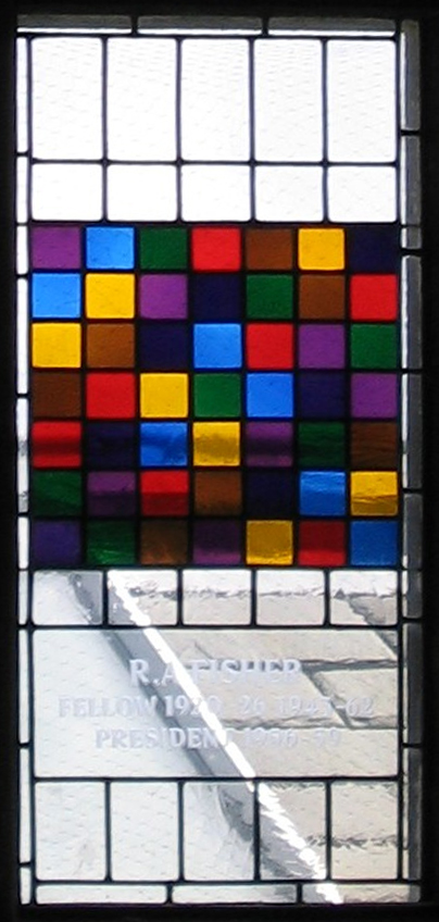
[edit]- ^ Busby, Mattha (27 June 2020). "Cambridge college to remove window commemorating eugenicist". The Guardian. Retrieved 2020-06-28.
- ^ Wallis, W. D.; George, J. C. (2011). Introduction to Combinatorics. CRC Press. p. 212. ISBN 978-1-4398-0623-4.
- ^ (Euler, 1782), pp. 90-91. From p. 90: "Pour cet effect nous reprenons le quarré latin fondamentel, qui, en omettant les exponsans, aura la forme suivante: …" (For this purpose, we take the fundamental Latin square, which, by omitting the exponents, will have the following form: …) From p. 91: "§.8 Ayant donc établi ce quarré latin, … " (§.8 Having thus established this Latin square, … ")
- ^ Euler, Leonhard (1782). "Recherches sur une nouvelle espèce de quarrés magiques" [Investigations into a new type of magic squares]. Verhandelingen Uitgegeven Door Het Zeeuwsch Genootschap der Wetenschappen te Vlissingen (Proceedings Published by the Zeeland Society of Sciences in Flushing [, Netherlands]) (in French). 9: 85–239. (Note: Euler first presented this memoir to the Imperial Academy of Sciences of St. Petersburg, Russia on 8 March 1779.)
- ^ Colbourn, Charles J.; Dinitz, Jeffrey H. (2007). Handbook of Combinatorial Designs (2nd ed.). CRC Press. p. 12. ISBN 9781420010541. Retrieved 28 March 2017.
- ^ McKay, Brendan D.; Meynert, Alison; Myrvold, Wendy (2007). "Small Latin squares, quasigroups, and loops". Journal of Combinatorial Designs. 15 (2): 98–119. doi:10.1002/jcd.20105. MR 2291523.
- ^ Euler, L. (1782). "Recherches sur une nouvelle espèce de quarrés magiques". Verhandelingen/Uitgegeven Door Het Zeeuwsch Genootschap der Wetenschappen te Vlissingen (9): 85–239.
- ^ Cayley, A. (1890). "On Latin Squares". Oxford Camb. Dublin Messenger of Math. 19: 85–239.
- ^ MacMahon, P.A. (1915). Combinatory Analysis. Cambridge University Press. p. 300.
- ^ Frolov, M. (1890). "Sur les permutations carrées". J. De Math. Spéc. IV: 8–11, 25–30.
- ^ Tarry, Gaston (1900). "Le Probléme de 36 Officiers". Compte Rendu de l'Association Française pour l'Avancement des Sciences. 1. Secrétariat de l'Association: 122–123.
- ^ Tarry, Gaston (1901). "Le Probléme de 36 Officiers". Compte Rendu de l'Association Française pour l'Avancement des Sciences. 2. Secrétariat de l'Association: 170–203.
- ^ Fisher, R.A.; Yates, F. (1934). "The 6 × 6 Latin squares". Proc. Cambridge Philos. Soc. 30 (4): 492–507. Bibcode:1934PCPS...30..492F. doi:10.1017/S0305004100012731. S2CID 120585553.
- ^ Schönhardt, E. (1930). "Über lateinische Quadrate und Unionen". J. Reine Angew. Math. 1930 (163): 183–230. doi:10.1515/crll.1930.163.183. S2CID 115237080.
- ^ Norton, H.W. (1939). "The 7 × 7 squares". Annals of Eugenics. 9 (3): 269–307. doi:10.1111/j.1469-1809.1939.tb02214.x.
- ^ Sade, A. (1951). "An omission in Norton's list of 7 × 7 squares". Ann. Math. Stat. 22 (2): 306–307. doi:10.1214/aoms/1177729654.
- ^ Saxena, P.N. (1951). "A simplified method of enumerating Latin squares by MacMahon's differential operators; II. The 7 × 7 Latin squares". J. Indian Soc. Agric. Statistics. 3: 24–79.
- ^ Preece, D.A. (1966). "Classifying Youden rectangles". J. Roy. Statist. Soc. Ser. B. 28: 118–130. doi:10.1111/j.2517-6161.1966.tb00625.x.
- ^ Brown, J.W. (1968). "Enumeration of Latin squares with application to order 8". Journal of Combinatorial Theory. 5 (2): 177–184. doi:10.1016/S0021-9800(68)80053-5.
- ^ Wells, M.B. (1967). "The number of Latin squares of order eight". Journal of Combinatorial Theory. 3: 98–99. doi:10.1016/S0021-9800(67)80021-8.
- ^ Kolesova, G.; Lam, C.W.H.; Thiel, L. (1990). "On the number of 8 × 8 Latin squares". Journal of Combinatorial Theory, Series A. 54: 143–148. doi:10.1016/0097-3165(90)90015-O.
- ^ Bammel, S.E.; Rothstein, J. (1975). "The number of 9 × 9 Latin squares". Discrete Mathematics. 11: 93–95. doi:10.1016/0012-365X(75)90108-9.
- ^ McKay, B.D.; Rogoyski, E. (1995). "Latin squares of order ten". Electronic Journal of Combinatorics. 2 N3: 4. doi:10.37236/1222.
- ^ McKay, B.D.; Wanless, I.M. (2005). "On the number of Latin squares". Ann. Comb. 9 (3): 335–344. doi:10.1007/s00026-005-0261-7. S2CID 7289396.
- ^ Dénes & Keedwell 1974, p. 128
- ^ Colbourn & Dinitz 2007, p. 136
- ^ Dénes & Keedwell 1974, p. 24
- ^ a b Dénes & Keedwell 1974, p. 126
- ^ van Lint & Wilson 1992, pp. 161-162
- ^ Jia-yu Shao; Wan-di Wei (1992). "A formula for the number of Latin squares". Discrete Mathematics. 110 (1–3): 293–296. doi:10.1016/0012-365x(92)90722-r.
- ^ Gyarfas, Andras; Sarkozy, Gabor N. (2012). "Rainbow matchings and partial transversals of Latin squares". arXiv:1208.5670 [CO math. CO].
- ^ a b Aharoni, Ron; Berger, Eli; Kotlar, Dani; Ziv, Ran (2017-01-04). "On a conjecture of Stein". Abhandlungen aus dem Mathematischen Seminar der Universität Hamburg. 87 (2): 203–211. arXiv:1605.01982. doi:10.1007/s12188-016-0160-3. ISSN 0025-5858. S2CID 119139740.
- ^ Stein, Sherman (1975-08-01). "Transversals of Latin squares and their generalizations". Pacific Journal of Mathematics. 59 (2): 567–575. doi:10.2140/pjm.1975.59.567. ISSN 0030-8730.
- ^ Koksma, Klaas K. (1969-07-01). "A lower bound for the order of a partial transversal in a latin square". Journal of Combinatorial Theory. 7 (1): 94–95. doi:10.1016/s0021-9800(69)80009-8. ISSN 0021-9800.
- ^ Woolbright, David E (1978-03-01). "An n × n Latin square has a transversal with at least n−n distinct symbols". Journal of Combinatorial Theory, Series A. 24 (2): 235–237. doi:10.1016/0097-3165(78)90009-2. ISSN 0097-3165.
- ^ Hatami, Pooya; Shor, Peter W. (2008-10-01). "A lower bound for the length of a partial transversal in a Latin square". Journal of Combinatorial Theory, Series A. 115 (7): 1103–1113. doi:10.1016/j.jcta.2008.01.002. ISSN 0097-3165.
- ^ Keevash, Peter; Pokrovskiy, Alexey; Sudakov, Benny; Yepremyan, Liana (2022-04-15). "New bounds for Ryser's conjecture and related problems". Transactions of the American Mathematical Society, Series B. 9 (8): 288–321. doi:10.1090/btran/92. hdl:20.500.11850/592212. ISSN 2330-0000.
- ^ Montgomery, Richard (2023). "A proof of the Ryser-Brualdi-Stein conjecture for large even n". arXiv:2310.19779 [math.CO].
- ^ Jacobson, M. T.; Matthews, P. (1996). "Generating uniformly distributed random latin squares". Journal of Combinatorial Designs. 4 (6): 405–437. doi:10.1002/(sici)1520-6610(1996)4:6<405::aid-jcd3>3.0.co;2-j.
- ^ Bailey, R.A. (2008). "6 Row-Column designs and 9 More about Latin squares". Design of Comparative Experiments. Cambridge University Press. ISBN 978-0-521-68357-9. MR 2422352.
- ^ Shah, Kirti R.; Sinha, Bikas K. (1989). "4 Row-Column Designs". Theory of Optimal Designs. Lecture Notes in Statistics. Vol. 54. Springer-Verlag. pp. 66–84. ISBN 0-387-96991-8. MR 1016151.
- ^ Colbourn, C.J.; Kløve, T.; Ling, A.C.H. (2004). "Permutation arrays for powerline communication". IEEE Trans. Inf. Theory. 50: 1289–1291. doi:10.1109/tit.2004.828150. S2CID 15920471.
- ^ Euler's revolution, New Scientist, 24 March 2007, pp 48–51
- ^ Huczynska, Sophie (2006). "Powerline communication and the 36 officers problem". Philosophical Transactions of the Royal Society A. 364 (1849): 3199–3214. Bibcode:2006RSPTA.364.3199H. doi:10.1098/rsta.2006.1885. PMID 17090455. S2CID 17662664.
- ^ C. Colbourn (1984). "The complexity of completing partial latin squares". Discrete Applied Mathematics. 8: 25–30. doi:10.1016/0166-218X(84)90075-1.
- ^ "The application of Latin square in agronomic research". Archived from the original on 2017-12-15. Retrieved 2017-04-02.
- ^ "Letters Patent Confering the SSC Arms". ssc.ca. Archived from the original on 2013-05-21.
- ^ The International Biometric Society Archived 2005-05-07 at the Wayback Machine
References
[edit]- Bailey, R.A. (2008). "6 Row-Column designs and 9 More about Latin squares". Design of Comparative Experiments. Cambridge University Press. ISBN 978-0-521-68357-9. MR 2422352.
- Dénes, J.; Keedwell, A. D. (1974). Latin squares and their applications. New York-London: Academic Press. p. 547. ISBN 0-12-209350-X. MR 0351850.
- Shah, Kirti R.; Sinha, Bikas K. (1989). "4 Row-Column Designs". Theory of Optimal Designs. Lecture Notes in Statistics. Vol. 54. Springer-Verlag. pp. 66–84. ISBN 0-387-96991-8. MR 1016151.
- van Lint, J. H.; Wilson, R. M. (1992). A Course in Combinatorics. Cambridge University Press. p. 157. ISBN 0-521-42260-4.
Further reading
[edit]- Dénes, J. H.; Keedwell, A. D. (1991). Latin squares: New developments in the theory and applications. Annals of Discrete Mathematics. Vol. 46. Paul Erdős (foreword). Amsterdam: Academic Press. ISBN 0-444-88899-3. MR 1096296.
- Hinkelmann, Klaus; Kempthorne, Oscar (2008). Design and Analysis of Experiments. Vol. I, II (Second ed.). Wiley. ISBN 978-0-470-38551-7. MR 2363107.
- Hinkelmann, Klaus; Kempthorne, Oscar (2008). Design and Analysis of Experiments, Volume I: Introduction to Experimental Design (Second ed.). Wiley. ISBN 978-0-471-72756-9. MR 2363107.
- Hinkelmann, Klaus; Kempthorne, Oscar (2005). Design and Analysis of Experiments, Volume 2: Advanced Experimental Design (First ed.). Wiley. ISBN 978-0-471-55177-5. MR 2129060.
- Knuth, Donald (2011). The Art of Computer Programming, Volume 4A: Combinatorial Algorithms, Part 1. Reading, Massachusetts: Addison-Wesley. ISBN 978-0-201-03804-0.
- Laywine, Charles F.; Mullen, Gary L. (1998). Discrete mathematics using Latin squares. Wiley-Interscience Series in Discrete Mathematics and Optimization. New York: John Wiley & Sons, Inc. ISBN 0-471-24064-8. MR 1644242.
- Shah, K. R.; Sinha, Bikas K. (1996). "Row-column designs". In S. Ghosh and C. R. Rao (ed.). Design and analysis of experiments. Handbook of Statistics. Vol. 13. Amsterdam: North-Holland Publishing Co. pp. 903–937. ISBN 0-444-82061-2. MR 1492586.
- Raghavarao, Damaraju (1988). Constructions and Combinatorial Problems in Design of Experiments (corrected reprint of the 1971 Wiley ed.). New York: Dover. ISBN 0-486-65685-3. MR 1102899.
- Street, Anne Penfold; Street, Deborah J. (1987). Combinatorics of Experimental Design. New York: Oxford University Press. ISBN 0-19-853256-3. MR 0908490.
- Berger, Paul D.; Maurer, Robert E.; Celli, Giovana B. (November 28, 2017). Experimental Design with Applications in Management, Engineering, and the Sciences (2nd edition (November 28, 2017) ed.). Springer. pp. 267–282.
External links
[edit]- Weisstein, Eric W. "Latin Square". MathWorld.
- Latin Squares in the Encyclopaedia of Mathematics
- Latin Squares in the Online Encyclopedia of Integer Sequences
| Scientific method | |
|---|---|
| Treatment and blocking | |
| Models and inference | |
| Designs Completely randomized | |
| Types |  | |
|---|---|---|
| Related shapes | ||
| Higher dimensional shapes | ||
| Classification | ||
| Related concepts | ||
| International | |
|---|---|
| National | |
| Other | |
Latin square
View on GrokipediaFundamentals
Definition
A Latin square of order is an array whose entries are symbols from a set of distinct elements, such that each symbol in appears exactly once in every row and exactly once in every column.[8] This structure ensures that the rows (or columns) form permutations of the symbol set .[9] The symbols need not be numbers; they can be any distinguishable objects, though conventionally labeled as through or letters of an alphabet.[8] For , the trivial Latin square consists of a single entry.[1] Order 2 yields two non-isomorphic Latin squares, both cyclic shifts or their transposes.[9] Higher orders produce exponentially more, with the number of Latin squares of order denoted , growing super-exponentially.[8]Reduced form and normalization
A reduced Latin square of order , also known as a normalized or standard form Latin square, uses symbols 1 through with the first row in natural order 1, 2, \dots, n and the first column similarly ordered 1, 2, \dots, n from top to bottom.[10][1][11] This canonical representation fixes the labeling of rows, columns, and symbols in specific positions to standardize the structure. Any Latin square can be isotoped to reduced form by permuting rows to position a chosen row first, relabeling symbols to order that row as 1 to , permuting columns to align the first row in sequence, and rearranging subsequent rows to sort the first column.[12] Isotopisms preserve the Latin property, ensuring every equivalence class under row, column, and symbol permutations contains exactly one reduced form, though distinct reduced squares may still be isotopic. Reduction aids enumeration by partitioning the set of all Latin squares. The total count satisfies , where denotes the number of reduced Latin squares of order .[5][13] This relation holds because each reduced square expands to distinct Latin squares via symbol permutation ( ways) and permutation of the rows after the first ( ways), with column adjustments maintaining the fixed first row order.[14] For small , , , , , and , reflecting increasing complexity in constructing such squares.[10]Historical Development
Origins in combinatorics
The combinatorial origins of Latin squares trace to puzzles involving constrained arrangements in the late 17th century. In 1694, French mathematician Jacques Ozanam presented a problem in Récréation mathématique requiring the arrangement of 16 court playing cards into a 4×4 grid such that each row and each column contains exactly one card of each suit and one of each rank (king, queen, jack, ace).[15] This construction is mathematically equivalent to a pair of orthogonal Latin squares of order 4, where one square encodes suits and the other ranks, demonstrating an early recognition of the structure's utility in ensuring balanced permutations without explicit formal definition.[16] Leonhard Euler formalized and expanded these ideas in the 18th century, naming the objects "carrés latins" in his 1782 memoir Recherches sur une nouvelle espèce de quarrés magiques.[17] Euler defined Latin squares as n×n arrays filled with n symbols, each appearing once per row and column, and explored their combinatorial properties, including the existence of orthogonal pairs that superimpose to form Graeco-Latin squares. He constructed such pairs for orders not congruent to 2 modulo 4 and applied them to magic square derivations.[15] A pivotal combinatorial challenge arose from Euler's 1782 "36 officers problem," which sought to arrange 36 officers—representing 6 ranks and 6 regiments—into a 6×6 formation where each row and column includes one officer of every rank and every regiment.[17] This requires two mutually orthogonal Latin squares of order 6, posing a question of existence that Euler conjectured impossible for orders of the form 4k+2, framing Latin squares within enumerative and existential combinatorics. The problem underscored the tension between construction methods and non-existence proofs, influencing subsequent studies in design theory.[18] Early enumerations by Euler included counts for small orders: 1 for n=2, 12 for n=3, and 576 for n=4, derived via systematic permutation checks, highlighting the rapid growth in combinatorial complexity.[15] These efforts established Latin squares as tools for modeling balanced incomplete block designs and scheduling, with roots in permutation group actions rather than algebraic structures initially.Euler's conjectures and resolutions
Leonhard Euler introduced the thirty-six officers problem in 1779, challenging the arrangement of 36 officers representing six ranks and six regiments into a 6×6 grid where each row and column includes exactly one officer per rank and one per regiment.[19] This arrangement equates to two orthogonal Latin squares of order 6, with one square encoding ranks and the other regiments. Euler concluded after extensive attempts that no solution exists for order 6.[20] Euler extended this observation into a broader conjecture in 1782, asserting that no pair of orthogonal Latin squares exists for any order , encompassing and higher such values, while allowing existence for other except powers of 2 under certain conditions.[21] The conjecture stemmed from Euler's failed constructions and partial enumerations, positing a structural incompatibility for these orders.[20] Gaston Tarry verified the impossibility for in 1900 through exhaustive manual enumeration of derangements and permutations, confirming no orthogonal pair exists despite the existence of Latin squares of that order.[17] This aligned with Euler's specific case but left the general claim unproven. The conjecture was refuted in 1959 when R. C. Bose, S. S. Shrikhande, and E. T. Parker constructed orthogonal pairs for and , using finite geometry and orthogonal arrays to bypass earlier limitations.[20] [22] Their methods, detailed in subsequent works, demonstrated existence for all except (trivially impossible) and , resolving the conjecture negatively while affirming the exceptional status of order 6.[20]Enumeration history and milestones
The enumeration of Latin squares originated with Leonhard Euler's manual counts in 1782, determining the numbers of reduced Latin squares (with the first row fixed as 1 to n in order) for orders 2 to 5 as 1, 1, 4, and 56, respectively.[23] These figures were independently verified by Arthur Cayley in 1890 using distinct methods.[23] In 1890, M. Frolov extended the effort to order 6, correctly enumerating 9408 reduced Latin squares of that order, though his count for order 7 proved erroneous.[23] Gaston Tarry confirmed Frolov's result for order 6 through exhaustive manual enumeration completed by 1901, a laborious process involving over 14 million cases to also disprove the existence of orthogonal mates for order 6.[23] P. R. McMahon applied an alternative recursive approach around the same era, reproducing the counts up to order 6 but replicating Frolov's error for order 7.[23] The first complete and accurate enumeration of reduced Latin squares of order 7, totaling 16,942,080, was achieved by A. Sade in the mid-20th century, marking a key milestone amid prior incomplete efforts like those of G. H. Norton.[23] Subsequent advances relied on computational methods; for instance, enumerations for orders 8 through 11 were obtained via systematic computer searches in the late 20th and early 21st centuries, with the order-11 count finalized around 2006 yielding over 10^{15} reduced squares.[5] These efforts highlighted recurring challenges, including computational complexity and historical discrepancies, underscoring the need for verification through independent algorithms.[24]Core Properties
Orthogonality and mutually orthogonal Latin squares
Two Latin squares and of order are orthogonal if the ordered pairs for comprise each possible ordered pair from the symbol sets exactly once.[25][26] This condition ensures that superimposing the squares yields a permutation of all symbol combinations without repetition.[27] A set of Latin squares of order forms a collection of mutually orthogonal Latin squares (MOLS) if every distinct pair in the set is orthogonal.[25][26] The maximum size of such a set, denoted , satisfies for all , with equality holding precisely when an affine plane of order exists.[26][28] When is a prime power, , and explicit constructions arise from the finite field .[28] One such construction defines the -th square (for ) by (with ), where indices and operations are over ; orthogonality follows because for distinct , the equation and solves uniquely for via field arithmetic, ensuring all pairs appear once.[28] For example, order (with ) yields two MOLS: where superimposition produces all 9 pairs exactly once.[28] For non-prime-power , ; notably, , as no pair of orthogonal Latin squares of order 6 exists, a result established through exhaustive enumeration and case analysis.[29] In general, for all with , and constructions via direct products or other combinatorial methods extend known sets for composite orders.[29] Sets of MOLS underpin orthogonal arrays of strength 2 and finite geometries, with MOLS equivalent to the resolution classes (minus one) of an affine plane's lines.[26]Equivalence, isotopism, and paratopism
Two Latin squares of order are isotopic if one can be obtained from the other by simultaneously permuting the rows via a permutation , the columns via , and the symbols via , yielding the transformed square .[24][30] The triple constitutes an isotopism, and the equivalence classes under this relation are termed isotopy classes.[24] An isotopism that maps a Latin square to itself is an autotopism.[30] A stricter notion, isomorphism, arises when , preserving the underlying quasigroup structure more rigidly; isomorphisms that fix the square are automorphisms.[24] Isotopy classes facilitate normalization, as every class contains a reduced (or normalized) representative with the first row and column fixed as .[24] However, isotopism does not account for reinterpretations of the square's axes, such as treating entries as rows or columns. Paratopism extends isotopism by incorporating parastrophism, which permutes the roles of the three coordinates (rows, columns, symbols) via an element of , yielding one of six parastrophes of the original square.[24][30] Formally, a paratopism is an element of the wreath product , acting as a parastrophism followed by an isotopism ; two squares are paratopic if one is the image of the other under such a map.[30] The resulting equivalence classes, known as main classes, group squares that represent the same combinatorial object under axis permutation and relabeling.[24] A paratopism fixing a square is an autoparatopism, and the set of all such forms a group under composition.[30] These relations are central to enumeration and classification, as direct counting of all Latin squares overcounts isomorphic or paratopic variants; for instance, the expected size of a main class is approximately .[24] Isotopism preserves properties like orthogonality within classes, while paratopism broaderens classification to capture quasigroup isotopy across parastrophes.[24]Asymptotic enumeration and existence theorems
The number of Latin squares of order is known exactly for , but asymptotic analysis provides tight bounds for large . These bounds are given by where the lower bound arises from counting completions of initial rows via permanents and Stirling's approximation, and the upper bound from partitioning into smaller structures.[23] The logarithm satisfies , indicating that grows roughly as .[23] [5] A foundational existence theorem, proved by Marshall Hall in 1945, states that any Latin rectangle with , where each symbol appears at most once per column, can be extended by adding further rows to form a full Latin square of order .[31] This constructive approach, relying on Hall's marriage theorem for systems of distinct representatives, confirms the existence of at least one Latin square for every positive integer order . For orthogonal Latin squares, pairs exist for all except , with constructions via finite fields for prime powers and other methods for composites, while non-existence for follows from exhaustive enumeration.[31] Asymptotic existence results include the construction of sets of mutually orthogonal Latin squares for sufficiently large , improving on trivial bounds and approaching the upper limit of achieved precisely when affine planes of order exist.[32]Transversals and Decompositions
Definition and basic existence results
A transversal in an n × n Latin square is a set of n cells containing exactly one cell from each row, exactly one from each column, and exactly one occurrence of each symbol.[33][34] Equivalently, for a permutation of , the cells form a transversal if the symbols are all distinct, where denotes the Latin square.[33] Transversals do not exist in every Latin square. A basic example is the cyclic Latin square defined by (with entries labeled to ) for even , which admits no transversal; this follows from the fact that any candidate set would require the sum of its symbols modulo to equal both (from distinct symbols) and (from row and column indices), leading to a contradiction for even .[34] More generally, the Cayley table of an abelian group of even order with exactly one element of order dividing 2 lacks a transversal.[33] A Latin square admits an orthogonal mate if and only if its cells can be partitioned into n disjoint transversals.[33][34] For group-based Latin squares, the Hall–Paige conjecture—resolved affirmatively in 2009—states that the Cayley table of a finite group G has a transversal if and only if every Sylow 2-subgroup of G is either trivial or non-cyclic.[33] It remains conjectured that every Latin square of odd order has at least one transversal, as proposed by Ryser in 1967 and consistent with computational checks up to order 11.[33][34]Partial transversals and the Ryser-Brualdi-Stein conjecture
A partial transversal of length in an Latin square is a set of cells with no two in the same row, no two in the same column, and no two containing the same symbol.[35] Such sets generalize full transversals, which achieve and thus select all rows, columns, and symbols exactly once; full transversals are equivalent to perfect matchings in the associated tripartite graph with parts for rows, columns, and symbols.[36] Partial transversals of maximal length provide insights into the structure of Latin squares, particularly regarding the existence of decompositions into transversals or orthogonal mates, as their scarcity can obstruct full coverings.[37] The Ryser-Brualdi-Stein conjecture states that every Latin square of order contains a partial transversal of length .[38] This claim emerged in the 1960s: Herbert Ryser conjectured in 1967 that all odd-order Latin squares admit full transversals, implying the case for odd , while Richard Brualdi independently proposed the guarantee for general , with Sherman Stein offering complementary observations on near-transversals.[36] For even , full transversals need not exist—as counterexamples include certain cyclic squares of order 2 modulo 4—making the bound the natural threshold.[39] The conjecture remains open in full generality, though verified computationally for small and proven for specific classes such as Latin squares derived from groups or prime power orders under additional conditions.[40] Established lower bounds guarantee partial transversals of length at least (up to constants) via probabilistic methods, with improvements to in some analyses, but these fall short of .[41] In 2023, Richard Montgomery established the conjecture for all sufficiently large even , using randomized algorithms and extremal graph theory to construct near-perfect matchings while avoiding symbol conflicts.[38] For odd , the result follows indirectly if Ryser's original conjecture holds, but direct proofs for leverage hall-like conditions in the symbol hypergraph.[36] Extensions and generalizations include bounds on the number of maximal partial transversals and their distribution in random Latin squares, where almost all instances exceed the conjectured minimum.[42] The conjecture intersects with rainbow matching problems in hypergraphs, where partial transversals correspond to color-avoiding selections, and failures would imply structural rigidity in Latin square permutations.[39] Ongoing research probes asymptotic densities and algorithmic constructibility, with implications for orthogonal array decompositions.[37]Rainbow matchings and recent advances
In the bipartite graph with partite sets corresponding to rows and columns of an Latin square, the entries define a proper edge-coloring using colors (the symbols), where each color class forms a perfect matching. A rainbow matching in this colored graph is a matching whose edges receive distinct colors, equivalent to a partial transversal in the Latin square: a set of positions with no two in the same row, column, or symbol. A perfect rainbow matching of size corresponds to a full transversal covering every row and column.[43][44] General results on rainbow matchings in properly edge-colored graphs provide bounds applicable to Latin squares. For instance, any such graph with contains a rainbow matching of size . In the Latin square setting, where and , this guarantees rainbow matchings larger than trivial bounds but falls short of for large . Stronger existential guarantees include Shor's 1982 result that every Latin square admits a partial transversal (rainbow matching) of size at least .[45][46] Recent advances have tightened these bounds significantly. In 2022, Keevash, Pokrovskiy, and Sudakov established that every Latin square has a partial transversal of size , improving prior logarithmic defect terms via probabilistic and algorithmic methods including the Rödl nibble. In 2023, Montgomery proved that sufficiently large Latin squares possess partial transversals of size exactly , nearing resolution of the Brualdi-Stein conjecture (every Latin square has a near-perfect partial transversal). The same work confirms the Ryser-Brualdi-Stein conjecture for large even orders, asserting that for each symbol, there exists a partial transversal avoiding that symbol and covering rows and columns. For random Latin squares, Kwan (2020) showed full transversals exist with high probability using the absorbing method, while Eberhard, Manners, and Mrazović (2023) quantified their asymptotic abundance as . These results leverage semi-random processes and analytic tools, advancing beyond deterministic constructions.[47][36][48]Computational Aspects
Construction algorithms
Latin squares of order exist for every positive integer , as demonstrated by the cyclic construction algorithm, which generates such a square by labeling rows, columns, and symbols from to and setting the entry in row , column to .[49] This method ensures each row is a cyclic shift of the previous, guaranteeing distinct symbols per row and column due to the properties of modular arithmetic.[50] More generally, the cyclic method allows shifting by positions where and , starting from an arbitrary first row permutation.[49] Another algebraic construction uses the Cayley table of any finite group of order : label rows and columns by group elements, and place the product (with symbols as group elements) at row , column .[51] This yields a Latin square because left (or right) multiplication by a fixed element is bijective in a group, ensuring each symbol appears once per row and column.[52] The cyclic group under addition recovers the basic cyclic square.[49] For composite orders with , the direct product construction combines Latin squares of orders and : replace each symbol in an order- square with an order- square scaled by the symbol index.[49] This recursively builds larger squares from smaller ones. For orders admitting a Steiner triple system (n ≡ 1 or 3 mod 6), a construction places the third triple element in off-diagonal positions defined by the triples, with diagonals as fixed points.[49] Computational algorithms, such as backtracking with constraint propagation, generate Latin squares by filling cells while enforcing row and column uniqueness, though efficiency decreases with .[53] For random generation, Markov chain methods like those of Jacobson and Matthews produce approximately uniform samples by transitioning between valid squares via symbol swaps.[54]Isomorphism testing and generation complexity
Testing whether two Latin squares of order are isomorphic—meaning one can be transformed into the other via independent permutations of rows, columns, and symbols—can be accomplished in quasi-polynomial time, specifically , through algorithms that leverage reductions to quasigroup isomorphism or structured graph isomorphism techniques.[55] This approach builds on advances in graph isomorphism solvers, which place the general problem in quasi-polynomial time, while specialized invariants for Latin squares, such as orthogonal mate existence or parastrophy classes, enable pruning in backtracking searches.[56] Polynomial-time reductions from full isomorphism to isotopism (permuting rows and columns without symbol relabeling) further streamline computation for structured cases.[55] A 2024 algorithm provides canonical labeling of Latin squares in average-case polynomial time by refining individualization-refinement methods tailored to the row-column-symbol permutation group, allowing isomorphism decisions by comparing canonical forms; this performs efficiently for randomly generated squares but may degrade for worst-case adversarial inputs.[57] Earlier practical methods, dating to 1978, employ group-theoretic invariants and backtracking to test quasigroup isomorphisms underlying Latin squares, achieving feasibility for moderate despite exponential worst-case behavior in symbol permutations.[56] Generating all non-isomorphic Latin squares of order involves enumerating under the action of the wreath product of symmetric groups , resulting in computational complexity dominated by the exponential growth in the number of reduced forms (with fixed first row and column), which exceeds asymptotically.[24] Exhaustive computational enumerations up to isomorphism have been completed for using optimized backtracking with isomorphism pruning via nauty-style canonicalization or invariant-based partitioning, yielding exact counts of isomorphism classes such as 2 for under full symmetry and larger figures for higher orders like thousands for .[58] For , non-isomorphic classes under various isotopism and paratopism actions were classified as early as 1967, but scaling beyond remains infeasible due to the superexponential size of the search space, estimated at over classes for .[59] Recent frameworks incorporate exact counting during generation via dynamic programming over partial rectangles, but full isomorphism resolution still requires post-processing with quasi-polynomial testers.[60]Applications
Statistics and experimental design
Latin square designs are employed in statistics to control for two sources of systematic variation in experiments, such as row and column effects in field trials. In this arrangement, treatments are assigned to experimental units so that each treatment appears exactly once in each row and each column of an n × n grid, where n is the number of treatments. This balances the design against heterogeneity in two directions, reducing error variance and increasing the precision of treatment effect estimates.[61] The statistical model for a Latin square design is typically yijk = μ + αi + τj + βk + εijk, where μ is the overall mean, αi the ith row effect, τj the jth treatment effect, βk the kth column effect, and εijk the random error term assumed normally distributed with mean zero and constant variance. Analysis of variance (ANOVA) partitions the total variation into components attributable to rows, columns, treatments, and residual error, testing for significant treatment effects after adjusting for blocking factors. This approach assumes additivity, meaning no interactions between row and column effects or with treatments; violations can lead to biased estimates.[62][63] Ronald A. Fisher pioneered the use of Latin squares in experimental design during the 1920s at Rothamsted Experimental Station, applying them to agricultural crop experiments to mitigate soil fertility gradients and other spatial biases. Fisher's 1935 book The Design of Experiments formalized their role in randomization and blocking, influencing modern factorial designs. In agronomy, for instance, a 5×5 Latin square was used in a 1929 Welsh hill planting to assess elevation effects on tree species, demonstrating practical efficacy in controlling topographic variation.[7][64][65] These designs are particularly valuable when experimental units are limited and two nuisance factors must be simultaneously blocked, outperforming randomized complete blocks in efficiency under balanced conditions. However, constructing orthogonal Latin squares or Graeco-Latin squares extends the method to additional factors, though availability decreases rapidly with order n. Limitations include the requirement for equal numbers of levels across factors and sensitivity to model misspecification, prompting alternatives like incomplete blocks for larger scales.[66][6]Error-correcting codes
Sets of mutually orthogonal Latin squares (MOLS) of order enable the construction of error-correcting codes by generating orthogonal arrays of index , strength 2, and runs, which define codes with minimum distance at least 3 for single-error correction.[67] A maximal set of MOLS corresponds to an affine plane of order , yielding codes capable of correcting up to errors where the code length is and dimension relates to the number of squares.[68] These structures exploit the orthogonality condition—where superimposed squares reveal all symbol pairs exactly times—to ensure that errors in codewords (rows of the array) can be detected and corrected via syndrome decoding based on row and column constraints.[69] Orthogonal Latin square (OLS) codes, derived from two or more MOLS, form a class of systematic multiple-error-correcting codes suitable for burst error patterns, as introduced in foundational work on finite geometries.[67] For instance, OLS codes based on pairs of orthogonal squares of order achieve a minimum distance of 4, enabling double-error correction, and have been extended to triple adjacent error correction by augmenting double-error-correcting variants with additional parity checks.[70] In memory applications, such as SRAM protection, OLS codes offer low check-bit overhead (e.g., 4 bits for 16 data bits in small orders) and simple encoder/decoder hardware, outperforming Hamming codes in multi-bit error scenarios due to their modularity.[71][72] Beyond classical uses, Latin squares underpin low-density parity-check (LDPC) codes via incidence matrices of quasigroups or orthogonal arrays, where rows represent variable nodes and columns check nodes, achieving near-Shannon-limit performance for certain parameters.[73] Recent extensions include quantum Latin squares for quantum error-correcting codes, preserving orthogonality under quantum operations to correct qubit errors, though these remain theoretical with focus on non-classical variants.[74][75] Empirical evaluations confirm OLS codes' efficacy in high-noise channels, with decoding complexity scaling linearly in for practical orders up to 256.Combinatorial puzzles
Sudoku is a prominent combinatorial puzzle derived from the Latin square structure, requiring the completion of a partially filled 9×9 grid such that each row, each column, and each of the nine 3×3 subgrids contains the digits 1 through 9 exactly once.[77] This imposes the no-repetition rule of a Latin square of order 9 alongside the block constraints, distinguishing it from plain Latin squares while embedding it within the broader combinatorial framework.[77] The puzzle's origins trace to number placement games, with modern Sudoku popularized in Japan in the late 1980s after earlier variants like Howard Garns's 1979 "Number Place."[78] More generally, Latin square puzzles challenge solvers to fill an n×n grid with n symbols such that no symbol repeats in any row or column, often starting from a partial configuration; these exist for various orders and symbol sets, serving as foundational logic exercises predating Sudoku by centuries, with examples appearing in Arabic mathematical texts over 700 years ago.[78] Variants extend the core mechanism, such as KenKen, which adds arithmetic constraints within irregularly shaped "cages" of cells while preserving the Latin square property, introduced by Tetsuya Miyamoto in 2004 to enhance logical deduction through operations like addition and multiplication.[79] Other adaptations include Strimko and Futoshiki, which incorporate stream connections or inequality rules, respectively, but all rely on the orthogonality and balance inherent to Latin squares for solvability.[80] These puzzles leverage the combinatorial richness of Latin squares, where the number of reduced Latin squares of order n grows factorially, ensuring diverse challenge levels.[81]Tournaments and scheduling
A tournament Latin square of order is defined as a Latin square satisfying the condition that implies .[82] This symmetry ensures that matches are undirected, with the pairing consistent across teams in each round. Such squares facilitate the construction of round-robin tournament schedules for teams over rounds, where row represents round , column team , and entry the opponent of team in that round.[82] In this setup, each row contains distinct symbols, guaranteeing that no team plays multiple opponents simultaneously, while each column's distinct symbols ensure every team faces each possible opponent exactly once across all rounds.[82] An entry indicates a bye for team in round , with the symmetry condition holding trivially in such cases. Consequently, each team receives exactly one bye, as symbol appears once per column . This structure suits tournaments where byes are acceptable, such as those with an odd number of teams, yielding rounds total.[82] Constructions of tournament Latin squares often rely on cyclic methods or group-based tables, such as the Cayley table of an abelian group adjusted for the symmetry requirement.[83] For enhanced balance, sets of mutually orthogonal Latin squares (MOLS) can overlay additional attributes, like venues or home/away assignments, ensuring no repeats in those factors across matches. For example, two orthogonal squares of order can schedule opponents and sites such that each team hosts each opponent exactly once.[84] In practice, these designs minimize biases like repeated pairings in consecutive rounds (via pandiagonal variants) or unbalanced travel, as explored in league scheduling algorithms.[82] Tournament Latin squares thus provide a combinatorial foundation for fair, verifiable schedules in sports leagues, with applications extending to non-sports events like bridge or whist tournaments requiring paired play without repetition.Agronomy and biological experiments
In agronomy, Latin square designs are applied to field trials to control spatial variability from two orthogonal blocking factors, such as fertility gradients along rows (e.g., downhill slopes) and columns (e.g., across-field moisture differences), thereby isolating treatment effects like fertilizer types or crop varieties more accurately than randomized complete block designs.[61] This bidirectional blocking reduces experimental error and increases precision, as demonstrated in a 2015 study on corn yield trials where Latin squares outperformed incomplete block designs by accounting for unrecognizable field gradients, yielding up to 20% higher statistical power in some configurations.[86] Ronald A. Fisher first advocated Latin squares for such agricultural experiments in the 1920s at Rothamsted Experimental Station, applying them to crop and forestry trials to subdivide variance sources via analysis of variance.[7] For example, Fisher used a Latin square in a 1924 replicated forestry experiment to evaluate tree species under elevation and positional effects. Practical implementations in agronomy include dividing plots into grids for testing soil amendments or irrigation methods, ensuring each treatment replicates once per row and column to balance environmental noise.[6] In dairy cattle grazing studies from the 1950s, Latin square change-over designs compared pasture qualities across animals and periods, achieving efficiency gains of 30-50% over non-balanced groupings by minimizing carryover effects.[87] Similarly, 1980 field trials on insect sex attractants employed Latin squares to counter wind direction and time-of-day biases, enabling clearer detection of lure efficacy differences.[88] In biological experiments beyond field settings, Latin squares facilitate crossover or repeated-measures designs to block two nuisance variables, such as subject heterogeneity and temporal sequences, in controlled lab or animal studies.[89] For instance, they minimize animal usage in nutritional trials by assigning diets to subjects over sequential periods, as in a 2003 poultry starch digestibility experiment where row blocks represented birds and column blocks represented time, reducing residual variance compared to incomplete Latin variants.[90] This approach is common in pharmacology and toxicology for dose-response assays, controlling inter-subject and intra-session variability while adhering to ethical constraints on sample sizes.[91] Overall, the design's orthogonality ensures estimable main effects, though assumptions of additive row and column impacts must hold for valid inference.[61]Heraldry and symbolic designs
The coat of arms granted to the Statistical Society of Canada on June 5, 1990, by the Canadian Heraldic Authority incorporates a 3×3 Latin square as its central charge, symbolizing the randomization and orthogonality inherent in statistical experimental design. The blazon describes it as "a Latin square chequy of nine Gules and Argent per bend reversed counterchanged," with each Argent (white) chequer charged with either a Gules (red) maple leaf or a Gules fleur-de-lis, ensuring each symbol appears exactly once per row and column.[92][93] This arrangement evokes the balanced distribution of treatments in Latin square-based blocking designs, aligning heraldry with the society's focus on empirical methodology.[94] In broader symbolic designs, Latin squares facilitate the creation of patterns where multiple sets of symbols are orthogonally superimposed without repetition in rows or columns, as seen in Greco-Latin squares for dual-layer representations. Such structures have potential utility in emblematic or graphical compositions requiring equitable element placement, though documented applications remain predominantly tied to statistical symbolism rather than standalone artistic or cultural motifs.[94] No widespread heraldic precedents beyond the Statistical Society of Canada exist in verified records, underscoring the niche integration of combinatorial mathematics into armorial bearings.[92]Recent interdisciplinary uses
In quantum information theory, quantum Latin squares have emerged as a generalization of classical Latin squares, where entries are unit vectors in an n-dimensional Hilbert space such that the inner product between distinct entries in the same row or column is zero.[95] Introduced in 2015, they facilitate the construction of unitary error bases and provide mathematical models for quantum phenomena including superposition, entanglement, teleportation, and dense coding.[96] Recent advancements, such as the 2025 construction of quantum Latin squares with all possible cardinalities from 1 to n^2, demonstrate their role in exploring quantum error-correcting codes beyond classical limits, with applications to fault-tolerant quantum computing. Non-classical orthogonal quantum Latin squares, verified to exist for orders up to 4 by 2025, enable more efficient quantum state discrimination and channel capacities compared to their classical counterparts.[97] In cryptography, Latin squares underpin recent image encryption schemes, particularly those integrating chaotic maps for enhanced diffusion and permutation. A 2021 algorithm employs Latin squares alongside random shifts and logistic maps to scramble pixel positions, achieving resistance to differential and statistical attacks with keys derived from initial chaotic conditions.[98] By 2022, transversals in Latin squares were used to generate pairs of orthogonal squares for bit-level substitutions in chaotic encryption, improving avalanche effects and key sensitivity in multimedia security.[99] Weighted-sum orthogonal Latin squares, explored in 2023 secret-sharing protocols, allow threshold access structures with verifiable reconstruction, leveraging the squares' orthogonality to distribute shares while minimizing computational overhead in distributed systems. Latin squares also inform network coding in wireless communications, where they represent bidirectional relaying maps satisfying exclusivity laws, as shown in models reducing decoding complexity for multi-user interference channels.[100] In biological data analysis, they structure microarray experiments for gene expression profiling, balancing treatments across replicates to isolate differential effects, with applications reported in 2024 reviews of algebraic extensions.[101] These uses highlight Latin squares' adaptability to quantum and computational constraints, though scalability remains challenged by enumeration complexity for higher orders.Generalizations
Latin rectangles and higher dimensions
A Latin rectangle is an r × n array (r ≤ n) filled with n symbols such that each symbol appears exactly once in every row and at most once in every column.[102][103] This structure generalizes the Latin square by allowing fewer rows, preserving the no-repeat condition only up to the partial height. The number of r × n Latin rectangles grows asymptotically as n!^r / e^{r(n-r)} times a subexponential factor, reflecting the combinatorial constraints on column distinctness.[103] Every r × n Latin rectangle can be extended by adding a new row to form an (r+1) × n Latin rectangle, a result proven using Hall's marriage theorem applied to bipartite matchings between symbols and columns avoiding prior entries.[104] Iterating this process yields a full n × n Latin square, ensuring completability in two dimensions regardless of the initial partial configuration, provided r ≤ n. This extendibility fails in higher dimensions, where partial arrays (hypercuboids) may resist completion to full hypercubes.[104][105] Higher-dimensional analogs, termed Latin hypercubes, extend the concept to d dimensions: a d-dimensional n × ⋯ × n array (order *n$, dimension d > 2) filled with symbols from 1 to n, where each line parallel to any coordinate axis contains each symbol exactly once.[106] For d=3, a Latin cube requires no repeats in rows, columns, or files (depth slices), generalizing Sudoku-like orthogonality to volumes.[107] Existence is guaranteed for prime power n via finite fields, but enumeration grows factorially with dimension, with the count for small d and n computable via backtracking or algebraic methods.[108] In dimensions d ≥ 3, maximal partial Latin hypercuboids—those not extendible by adding a slice perpendicular to one axis—exist, contrasting the two-dimensional case; for instance, certain n × n × k cuboids with k < n cannot be completed.[105][109] These structures underpin generalizations like orthogonal arrays and support applications in multi-way experimental designs, where symbols represent factor levels across multiple indices.[106]Quasigroups and algebraic structures
A Latin square of order on a symbol set of size serves as the Cayley table for a quasigroup of order . In this representation, the rows and columns are indexed by the elements of the quasigroup , and the entry in row , column is the product , ensuring each symbol appears exactly once in each row and column due to the bijectivity of left and right multiplications. Conversely, any such Latin square defines a quasigroup operation on the index set by assigning the entry value as the product.[110][10] A quasigroup is a magma (set with binary operation) where, for all , the equations and admit unique solutions ; this guarantees the Latin square property without requiring associativity or an identity element. Loops extend quasigroups by including a two-sided identity satisfying for all , corresponding to a Latin square where the -row and -column replicate the symbol order (up to labeling). Groups, as associative loops with inverses, produce Latin squares that satisfy the group axioms, such as the cyclic group under addition modulo , whose table consists of cyclic row shifts.[10][111][112] Equivalence relations on these structures account for relabelings: two quasigroups are isomorphic via a bijection preserving the operation (), while isotopy relaxes this by allowing independent bijections on domain, range, and codomain such that ; the corresponding Latin squares are obtained by permuting rows (), columns (), and symbols (). Isotopic quasigroups preserve solvability but may differ structurally, whereas paratopisms further permute operation roles (e.g., to left division tables), yielding additional Latin square variants from the same quasigroup. These notions classify Latin squares up to algebraic similarity, with reduced forms fixing the first row and column to standardize comparisons.[110][10] Specialized quasigroup subclasses yield Latin squares with enhanced properties: idempotent quasigroups () produce squares with constant diagonals; commutative quasigroups give symmetric tables. Loops satisfying identities like Moufang laws (, etc.) form structures like Moufang loops, whose tables support orthogonal mate constructions relevant to finite geometries. The enumeration of small-order quasigroups and loops, via computational enumeration of reduced Latin squares, reveals growth rates: for order 5, there are 161 quasigroups up to isomorphism, including 2 groups and 12 loops.[10][112][113]Frequency squares and incomplete variants
A frequency square of order and type is an array filled with distinct symbols such that symbol appears exactly times in every row and every column, where .[114] This structure reduces to a standard Latin square when and each .[115] Frequency squares were introduced by Percy MacMahon in 1898 under the term "quasi-Latin square" to extend combinatorial properties beyond uniform symbol occurrences.[114] Two frequency squares of the same order and type are mutually orthogonal if, when superimposed, every ordered pair of symbols appears together in exactly cells.[116] The maximum number of mutually orthogonal frequency squares sharing the same type is bounded by the minimum , analogous to the bound for Latin squares.[117] Binary frequency squares, where and symbols appear with frequencies and , have been enumerated for small , revealing connections to balanced incomplete block designs.[115] Incomplete variants of Latin squares include partial Latin squares, which are arrays with some cells filled such that no symbol repeats in any row or column among the filled entries, but fewer than cells are occupied.[118] These differ from full Latin squares by allowing vacancies, and their completability—extension to a full Latin square without altering filled cells—remains a central problem, with algorithms succeeding for fill rates up to 50% in orders up to 10 but failing deterministically for higher densities in larger orders.[119] In experimental design, incomplete Latin squares, such as Youden squares derived by omitting one row from a full square, provide unbiased error estimates for factorial treatments when full replication is infeasible.[120] Balanced incomplete Latin square designs extend this by ensuring every pair of treatments appears together a constant number of times across blocks, addressing limitations in row-column blocking for incomplete data.[121]Open Problems
Unresolved conjectures on MOLS
The maximum number of mutually orthogonal Latin squares (MOLS) of order satisfies for all , with equality holding if and only if an affine plane of order exists.[122][123] Constructions achieving are known precisely when is a prime power, via the vector space structure over the finite field .[124] For non-prime-power , no such complete sets are known, and non-existence is established for small cases like (where ) through exhaustive enumeration.[125] A longstanding conjecture posits that if and only if is a prime power, implying that affine planes—and thus complete MOLS sets—do not exist for other orders.[126] This remains unresolved, as no counterexamples have been found despite extensive searches, and theoretical obstructions like the Bruck-Ryser-Chowla theorem rule out projective planes (from which affine planes can sometimes be derived) for certain non-prime-power or that are not sums of two squares.[127] However, the conjecture lacks a general proof, with the status of open for many composite such as 15, 21, and 33, where upper bounds below exist but fall short of confirming the gap.[128] Lower bounds on for general are also subjects of conjecture and refinement. The MacNeish-Mann conjecture, which posits that is at least the minimum of over the prime factorization , provides a constructive lower bound via tensor products but is not sharp; stronger asymptotic estimates suggest for some constant , yet the precise growth rate remains conjectural.[128][129] Specific values like and are known to be small (e.g., but far below 9), fueling related questions on whether can exceed certain thresholds tied to factorization minima.[125] These issues persist due to the combinatorial explosion in verifying orthogonality for large , with computational efforts confirming bounds up to modest orders but leaving higher cases theoretically indeterminate.[127]Transversal existence for specific orders
Ryser's conjecture posits that every Latin square of odd order possesses at least one transversal, with the number of transversals being odd in such cases.[130] This remains unproven, though computational verification confirms its validity for all odd orders up to 9.[130] No counterexamples exist for odd orders, distinguishing them from even orders where transversals are absent in certain constructions.[131] For even orders, Latin squares without transversals are well-documented, beginning with order 2. The unique (up to isomorphism) Latin square of order 2, given by the rows , lacks a transversal, as both possible permutations yield repeated symbols.[131] Similarly, the Cayley table of the cyclic group of even order admits no transversal, a consequence of the group's structure lacking a complete set of representatives for the cosets of its Sylow 2-subgroup.[131] This extends to group-based Latin squares of even order with cyclic Sylow 2-subgroups, which are transversal-free.[132] Constructions yielding transversal-free Latin squares proliferate for larger even orders, such as . For instance, back-circulant Latin squares similar to the cyclic group table of order can be modified to eliminate transversals while preserving the Latin property, with the number of such distinct species growing exponentially as for even .[133] Every Latin square of even order has an even number of transversals (possibly zero), reinforcing the parity distinction from odd orders.[34] These results underscore that transversal existence is not guaranteed for even orders, unlike the conjectured universality for odd orders.Classification challenges for larger orders
The classification of Latin squares of order up to isomorphism—determining the number of distinct classes under relabeling of rows, columns, and symbols—has been achieved computationally for , but encounters formidable barriers for higher orders due to the explosive growth in the underlying combinatorial space. For , there are precisely isomorphism classes, enumerated via optimized backtracking algorithms that prune invalid partial fillings and exploit symmetries to avoid redundant computations. This required extensive parallel processing over months on high-performance clusters, highlighting the resource intensity even at this scale.[134] Extending such enumerations to proves infeasible with current methods, as the total number of Latin squares alone exceeds , and partitioning them into isomorphism classes demands evaluating orbits under the action of the symmetric group , whose order is , vastly complicating direct application of tools like Burnside's lemma. Algorithms rely on generating canonical representatives—unique forms under isomorphism via lexicographic minimization—but the search tree branches factorially at each step, with symmetry-breaking techniques (e.g., fixing initial rows and testing stabilizers) insufficient to tame the complexity beyond . No complete count of isomorphism classes exists for , despite partial results for subclasses like reduced or diagonal Latin squares.[24] For even larger , classification shifts from exact enumeration to probabilistic or asymptotic approximations, as exhaustive computation becomes asymptotically harder than #P-complete problems like counting perfect matchings in bipartite graphs, given the structural analogies to quasigroup multiplication tables. Key obstacles include managing memory for partial enumerations (gigabytes for , petabytes projected for ) and developing isomorphism-invariant descriptors robust to the diversity of square types, such as those isotopic to groups versus parastrophes of projective planes. Progress hinges on advances in algebraic invariants (e.g., deriving quasigroup properties) or machine learning for pattern detection in random samples, but full structural classification remains unattainable, limiting insights into phenomena like the distribution of orthogonal mates or transversal counts across classes.[135]References
- https://www.[researchgate](/page/ResearchGate).net/publication/301221246_ERROR_CORRECTING_CODE_USING_LATIN_SQUARE
- https://www.[researchgate](/page/ResearchGate).net/publication/268322374_Designing_tournaments_with_the_aid_of_Latin_squares_A_presentation_of_old_and_new_results