Hubbry Logo
Merge sortMerge sortMain
Open search
Merge sort
Community hub
Merge sort
logo
8 pages, 0 posts
0 subscribers
Be the first to start a discussion here.
Contribute something
Merge sort
Merge sort
from Wikipedia
Merge sort
An example of merge sort. First, divide the list into the smallest unit (1 element), then compare each element with the adjacent list to sort and merge the two adjacent lists. Finally, all the elements are sorted and merged.
ClassSorting algorithm
Data structureArray
Worst-case performance
Best-case performance typical, natural variant
Average performance
Worst-case space complexity total with auxiliary, auxiliary with linked lists[1]

In computer science, merge sort (also commonly spelled as mergesort and as merge-sort[2]) is an efficient, general-purpose, and comparison-based sorting algorithm. Most implementations of merge sort are stable, which means that the relative order of equal elements is the same between the input and output. Merge sort is a divide-and-conquer algorithm that was invented by John von Neumann in 1945.[3] A detailed description and analysis of bottom-up merge sort appeared in a report by Goldstine and von Neumann as early as 1948.[4]

Algorithm

[edit]

Conceptually, a merge sort works as follows:

  1. Divide the unsorted list into n sub-lists, each containing one element (a list of one element is considered sorted).
  2. Repeatedly merge sublists to produce new sorted sublists until there is only one sublist remaining. This will be the sorted list.

Top-down implementation

[edit]

Example C-like code using indices for top-down merge sort algorithm that recursively splits the list (called runs in this example) into sublists until sublist size is 1, then merges those sublists to produce a sorted list. The copy back step is avoided with alternating the direction of the merge with each level of recursion (except for an initial one-time copy, that can be avoided too).

As a simple example, consider an array with two elements. The elements are copied to B[], then merged back to A[]. If there are four elements, when the bottom of the recursion level is reached, single element runs from A[] are merged to B[], and then at the next higher level of recursion, those two-element runs are merged to A[]. This pattern continues with each level of recursion.

// Array A[] has the items to sort; array B[] is a work array.
void TopDownMergeSort(A[], B[], n)
{
    CopyArray(A, 0, n, B);           // one time copy of A[] to B[]
    TopDownSplitMerge(A, 0, n, B);   // sort data from B[] into A[]
}

// Split A[] into 2 runs, sort both runs into B[], merge both runs from B[] to A[]
// iBegin is inclusive; iEnd is exclusive (A[iEnd] is not in the set).
void TopDownSplitMerge(B[], iBegin, iEnd, A[])
{
    if (iEnd - iBegin <= 1)                     // if run size == 1
        return;                                 //   consider it sorted
    // split the run longer than 1 item into halves
    iMiddle = (iEnd + iBegin) / 2;              // iMiddle = mid point
    // recursively sort both runs from array A[] into B[]
    TopDownSplitMerge(A, iBegin,  iMiddle, B);  // sort the left  run
    TopDownSplitMerge(A, iMiddle,    iEnd, B);  // sort the right run
    // merge the resulting runs from array B[] into A[]
    TopDownMerge(B, iBegin, iMiddle, iEnd, A);
}

//  Left source half is A[ iBegin:iMiddle-1].
// Right source half is A[iMiddle:iEnd-1   ].
// Result is            B[ iBegin:iEnd-1   ].
void TopDownMerge(B[], iBegin, iMiddle, iEnd, A[])
{
    i = iBegin, j = iMiddle;
 
    // While there are elements in the left or right runs...
    for (k = iBegin; k < iEnd; k++) {
        // If left run head exists and is <= existing right run head.
        if (i < iMiddle && (j >= iEnd || A[i] <= A[j])) {
            B[k] = A[i];
            i = i + 1;
        } else {
            B[k] = A[j];
            j = j + 1;
        }
    }
}

void CopyArray(A[], iBegin, iEnd, B[])
{
    for (k = iBegin; k < iEnd; k++)
        B[k] = A[k];
}

Sorting the entire array is accomplished by TopDownMergeSort(A, B, length(A)).

Bottom-up implementation

[edit]

Example C-like code using indices for bottom-up merge sort algorithm which treats the list as an array of n sublists (called runs in this example) of size 1, and iteratively merges sub-lists back and forth between two buffers:

// array A[] has the items to sort; array B[] is a work array
void BottomUpMergeSort(A[], B[], n)
{
    // Each 1-element run in A is already "sorted".
    // Make successively longer sorted runs of length 2, 4, 8, 16... until the whole array is sorted.
    for (width = 1; width < n; width = 2 * width)
    {
        // Array A is full of runs of length width.
        for (i = 0; i < n; i = i + 2 * width)
        {
            // Merge two runs: A[i:i+width-1] and A[i+width:i+2*width-1] to B[]
            // or copy A[i:n-1] to B[] ( if (i+width >= n) )
            BottomUpMerge(A, i, min(i+width, n), min(i+2*width, n), B);
        }
        // Now work array B is full of runs of length 2*width.
        // Copy array B to array A for the next iteration.
        // A more efficient implementation would swap the roles of A and B.
        CopyArray(B, A, n);
        // Now array A is full of runs of length 2*width.
    }
}

//  Left run is A[iLeft :iRight-1].
// Right run is A[iRight:iEnd-1  ].
void BottomUpMerge(A[], iLeft, iRight, iEnd, B[])
{
    i = iLeft, j = iRight;
    // While there are elements in the left or right runs...
    for (k = iLeft; k < iEnd; k++) {
        // If left run head exists and is <= existing right run head.
        if (i < iRight && (j >= iEnd || A[i] <= A[j])) {
            B[k] = A[i];
            i = i + 1;
        } else {
            B[k] = A[j];
            j = j + 1;    
        }
    } 
}

void CopyArray(B[], A[], n)
{
    for (i = 0; i < n; i++)
        A[i] = B[i];
}

Top-down implementation using lists

[edit]

Pseudocode for top-down merge sort algorithm which recursively divides the input list into smaller sublists until the sublists are trivially sorted, and then merges the sublists while returning up the call chain.

function merge_sort(list m) is
    // Base case. A list of zero or one elements is sorted, by definition.
    if length of m ≤ 1 then
        return m

    // Recursive case. First, divide the list into equal-sized sublists
    // consisting of the first half and second half of the list.
    // This assumes lists start at index 0.
    var left := empty list
    var right := empty list
    for each x with index i in m do
        if i < (length of m)/2 then
            add x to left
        else
            add x to right

    // Recursively sort both sublists.
    left := merge_sort(left)
    right := merge_sort(right)

    // Then merge the now-sorted sublists.
    return merge(left, right)

In this example, the merge function merges the left and right sublists.
function merge(left, right) is
    var result := empty list

    while left is not empty and right is not empty do
        if first(left) ≤ first(right) then
            append first(left) to result
            left := rest(left)
        else
            append first(right) to result
            right := rest(right)

    // Either left or right may have elements left; consume them.
    // (Only one of the following loops will actually be entered.)
    while left is not empty do
        append first(left) to result
        left := rest(left)
    while right is not empty do
        append first(right) to result
        right := rest(right)
    return result

Bottom-up implementation using lists

[edit]

Pseudocode for bottom-up merge sort algorithm which uses a small fixed size array of references to nodes, where array[i] is either a reference to a list of size 2i or nil. node is a reference or pointer to a node. The merge() function would be similar to the one shown in the top-down merge lists example, it merges two already sorted lists, and handles empty lists. In this case, merge() would use node for its input parameters and return value.

function merge_sort(node head) is
    // return if empty list
    if head = nil then
        return nil
    var node array[32]; initially all nil
    var node result
    var node next
    var int  i
    result := head
    // merge nodes into array
    while result ≠ nil do
        next := result.next;
        result.next := nil
        for (i = 0; (i < 32) && (array[i] ≠ nil); i += 1) do
            result := merge(array[i], result)
            array[i] := nil
        // do not go past end of array
        if i = 32 then
            i -= 1
        array[i] := result
        result := next
    // merge array into single list
    result := nil
    for (i = 0; i < 32; i += 1) do
        result := merge(array[i], result)
    return result

Top-down implementation in a declarative style

[edit]

Haskell-like pseudocode, showing how merge sort can be implemented in such a language using constructs and ideas from functional programming.

mergeSort :: Ord a => [a] -> [a]
mergeSort []  = []
mergeSort [x] = [x]
mergeSort xs  = merge (mergeSort l, mergeSort r)
  where (l, r) = splitAt (length xs `div` 2) xs

merge :: Ord a => ([a], [a]) -> [a]
merge ([], xs) = xs
merge (xs, []) = xs
merge (x:xs, y:ys) | x <= y    = x : merge(xs, y:ys)
                   | otherwise = y : merge(x:xs, ys)

Analysis

[edit]
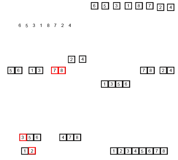
A recursive merge sort algorithm used to sort an array of 7 integer values. These are the steps a human would take to emulate merge sort (top-down).

In sorting n objects, merge sort has an average and worst-case performance of O(n log n) comparisons. If the running time (number of comparisons) of merge sort for a list of length n is T(n), then the recurrence relation T(n) = 2T(n/2) + n follows from the definition of the algorithm (apply the algorithm to two lists of half the size of the original list, and add the n steps taken to merge the resulting two lists).[5] The closed form follows from the master theorem for divide-and-conquer recurrences.

The number of comparisons made by merge sort in the worst case is given by the sorting numbers. These numbers are equal to or slightly smaller than (n ⌈lg n⌉ − 2⌈lg n + 1), which is between (n lg nn + 1) and (n lg n + n + O(lg n)).[6] Merge sort's best case takes about half as many iterations as its worst case.[7]

For large n and a randomly ordered input list, merge sort's expected (average) number of comparisons approaches α·n fewer than the worst case, where

In the worst case, merge sort uses approximately 39% fewer comparisons than quicksort does in its average case, and in terms of moves, merge sort's worst case complexity is O(n log n) - the same complexity as quicksort's best case.[7]

Merge sort is more efficient than quicksort for some types of lists if the data to be sorted can only be efficiently accessed sequentially, and is thus popular in languages such as Lisp, where sequentially accessed data structures are very common. Unlike some (efficient) implementations of quicksort, merge sort is a stable sort.

Merge sort's most common implementation does not sort in place;[8] therefore, the memory size of the input must be allocated for the sorted output to be stored in (see below for variations that need only n/2 extra spaces).

Natural merge sort

[edit]

A natural merge sort is similar to a bottom-up merge sort except that any naturally occurring runs (sorted sequences) in the input are exploited. Both monotonic and bitonic (alternating up/down) runs may be exploited, with lists (or equivalently tapes or files) being convenient data structures (used as FIFO queues or LIFO stacks).[9] In the bottom-up merge sort, the starting point assumes each run is one item long. In practice, random input data will have many short runs that just happen to be sorted. In the typical case, the natural merge sort may not need as many passes because there are fewer runs to merge. In the best case, the input is already sorted (i.e., is one run), so the natural merge sort need only make one pass through the data. In many practical cases, long natural runs are present, and for that reason natural merge sort is exploited as the key component of Timsort. Example:

Start       :  3  4  2  1  7  5  8  9  0  6
Select runs : (3  4)(2)(1  7)(5  8  9)(0  6)
Merge       : (2  3  4)(1  5  7  8  9)(0  6)
Merge       : (1  2  3  4  5  7  8  9)(0  6)
Merge       : (0  1  2  3  4  5  6  7  8  9)

Formally, the natural merge sort is said to be Runs-optimal, where is the number of runs in , minus one.

Tournament replacement selection sorts are used to gather the initial runs for external sorting algorithms.

Ping-pong merge sort

[edit]

Instead of merging two blocks at a time, a ping-pong merge merges four blocks at a time. The four sorted blocks are merged simultaneously to auxiliary space into two sorted blocks, then the two sorted blocks are merged back to main memory. Doing so omits the copy operation and reduces the total number of moves by half. An early public domain implementation of a four-at-once merge was by WikiSort in 2014, the method was later that year described as an optimization for patience sorting and named a ping-pong merge.[10][11] Quadsort implemented the method in 2020 and named it a quad merge.[12]

In-place merge sort

[edit]

One drawback of merge sort, when implemented on arrays, is its O(n) working memory requirement. Several methods to reduce memory or make merge sort fully in-place have been suggested:

  • Kronrod (1969) suggested an alternative version of merge sort that uses constant additional space.
  • Katajainen et al. present an algorithm that requires a constant amount of working memory: enough storage space to hold one element of the input array, and additional space to hold O(1) pointers into the input array. They achieve an O(n log n) time bound with small constants, but their algorithm is not stable.[13]
  • Several attempts have been made at producing an in-place merge algorithm that can be combined with a standard (top-down or bottom-up) merge sort to produce an in-place merge sort. In this case, the notion of "in-place" can be relaxed to mean "taking logarithmic stack space", because standard merge sort requires that amount of space for its own stack usage. It was shown by Geffert et al. that in-place, stable merging is possible in O(n log n) time using a constant amount of scratch space, but their algorithm is complicated and has high constant factors: merging arrays of length n and m can take 5n + 12m + o(m) moves.[14] This high constant factor and complicated in-place algorithm was made simpler and easier to understand. Bing-Chao Huang and Michael A. Langston[15] presented a straightforward linear time algorithm practical in-place merge to merge a sorted list using fixed amount of additional space. They both have used the work of Kronrod and others. It merges in linear time and constant extra space. The algorithm takes little more average time than standard merge sort algorithms, free to exploit O(n) temporary extra memory cells, by less than a factor of two. Though the algorithm is much faster in a practical way, it is unstable for some lists. But using similar concepts, they have been able to solve this problem. Other in-place algorithms include SymMerge, which takes O((n + m) log (n + m)) time in total and is stable.[16] Plugging such an algorithm into merge sort increases its complexity to the non-linearithmic, but still quasilinear, O(n (log n)2).
  • Many applications of external sorting use a form of merge sorting where the input gets split up to a higher number of sublists, ideally to a number for which merging them still makes the currently processed set of pages fit into main memory.
  • A modern stable, linear, and in-place merge variant is block merge sort, which creates a section of unique values to use as swap space.
  • The space overhead can be reduced to O(√n) by using binary searches and rotations.[17] This method is employed by the C++ STL library and quadsort.[12]
  • An alternative to reduce the copying into multiple lists is to associate a new field of information with each key (the elements in m are called keys). This field will be used to link the keys and any associated information together in a sorted list (a key and its related information is called a record). Then the merging of the sorted lists proceeds by changing the link values; no records need to be moved at all. A field which contains only a link will generally be smaller than an entire record so less space will also be used. This is a standard sorting technique, not restricted to merge sort.
  • A simple way to reduce the space overhead to n/2 is to maintain left and right as a combined structure, copy only the left part of m into temporary space, and to direct the merge routine to place the merged output into m. With this version it is better to allocate the temporary space outside the merge routine, so that only one allocation is needed. The excessive copying mentioned previously is also mitigated, since the last pair of lines before the return result statement (function merge in the pseudo code above) become superfluous.

Use with tape drives

[edit]
Merge sort type algorithms allowed large data sets to be sorted on early computers that had small random access memories by modern standards. Records were stored on magnetic tape and processed on banks of magnetic tape drives, such as these IBM 729s.

An external merge sort is practical to run using disk or tape drives when the data to be sorted is too large to fit into memory. External sorting explains how merge sort is implemented with disk drives. A typical tape drive sort uses four tape drives. All I/O is sequential (except for rewinds at the end of each pass). A minimal implementation can get by with just two record buffers and a few program variables.

Naming the four tape drives as A, B, C, D, with the original data on A, and using only two record buffers, the algorithm is similar to the bottom-up implementation, using pairs of tape drives instead of arrays in memory. The basic algorithm can be described as follows:

  1. Merge pairs of records from A; writing two-record sublists alternately to C and D.
  2. Merge two-record sublists from C and D into four-record sublists; writing these alternately to A and B.
  3. Merge four-record sublists from A and B into eight-record sublists; writing these alternately to C and D
  4. Repeat until you have one list containing all the data, sorted—in log2(n) passes.

Instead of starting with very short runs, usually a hybrid algorithm is used, where the initial pass will read many records into memory, do an internal sort to create a long run, and then distribute those long runs onto the output set. The step avoids many early passes. For example, an internal sort of 1024 records will save nine passes. The internal sort is often large because it has such a benefit. In fact, there are techniques that can make the initial runs longer than the available internal memory. One of them, the Knuth's 'snowplow' (based on a binary min-heap), generates runs twice as long (on average) as a size of memory used.[18]

With some overhead, the above algorithm can be modified to use three tapes. O(n log n) running time can also be achieved using two queues, or a stack and a queue, or three stacks. In the other direction, using k > two tapes (and O(k) items in memory), we can reduce the number of tape operations in O(log k) times by using a k/2-way merge.

A more sophisticated merge sort that optimizes tape (and disk) drive usage is the polyphase merge sort.

Optimizing merge sort

[edit]
Tiled merge sort applied to an array of random integers. The horizontal axis is the array index and the vertical axis is the integer.

On modern computers, locality of reference can be of paramount importance in software optimization, because multilevel memory hierarchies are used. Cache-aware versions of the merge sort algorithm, whose operations have been specifically chosen to minimize the movement of pages in and out of a machine's memory cache, have been proposed. For example, the tiled merge sort algorithm stops partitioning subarrays when subarrays of size S are reached, where S is the number of data items fitting into a CPU's cache. Each of these subarrays is sorted with an in-place sorting algorithm such as insertion sort, to discourage memory swaps, and normal merge sort is then completed in the standard recursive fashion. This algorithm has demonstrated better performance[example needed] on machines that benefit from cache optimization. (LaMarca & Ladner 1997)

Parallel merge sort

[edit]

Merge sort parallelizes well due to the use of the divide-and-conquer method. Several different parallel variants of the algorithm have been developed over the years. Some parallel merge sort algorithms are strongly related to the sequential top-down merge algorithm while others have a different general structure and use the K-way merge method.

Merge sort with parallel recursion

[edit]

The sequential merge sort procedure can be described in two phases, the divide phase and the merge phase. The first consists of many recursive calls that repeatedly perform the same division process until the subsequences are trivially sorted (containing one or no element). An intuitive approach is the parallelization of those recursive calls.[19] Following pseudocode describes the merge sort with parallel recursion using the fork and join keywords:

// Sort elements lo through hi (exclusive) of array A.
algorithm mergesort(A, lo, hi) is
    if lo+1 < hi then  // Two or more elements.
        mid := ⌊(lo + hi) / 2⌋
        fork mergesort(A, lo, mid)
        mergesort(A, mid, hi)
        join
        merge(A, lo, mid, hi)

This algorithm is the trivial modification of the sequential version and does not parallelize well. Therefore, its speedup is not very impressive. It has a span of , which is only an improvement of compared to the sequential version (see Introduction to Algorithms). This is mainly due to the sequential merge method, as it is the bottleneck of the parallel executions.

Merge sort with parallel merging

[edit]

Better parallelism can be achieved by using a parallel merge algorithm. Cormen et al. present a binary variant that merges two sorted sub-sequences into one sorted output sequence.[19]

In one of the sequences (the longer one if unequal length), the element of the middle index is selected. Its position in the other sequence is determined in such a way that this sequence would remain sorted if this element were inserted at this position. Thus, one knows how many other elements from both sequences are smaller and the position of the selected element in the output sequence can be calculated. For the partial sequences of the smaller and larger elements created in this way, the merge algorithm is again executed in parallel until the base case of the recursion is reached.

The following pseudocode shows the modified parallel merge sort method using the parallel merge algorithm (adopted from Cormen et al.).

/**
 * A: Input array
 * B: Output array
 * lo: lower bound
 * hi: upper bound
 * off: offset
 */
algorithm parallelMergesort(A, lo, hi, B, off) is
    len := hi - lo + 1
    if len == 1 then
        B[off] := A[lo]
    else let T[1..len] be a new array
        mid := ⌊(lo + hi) / 2⌋ 
        mid' := mid - lo + 1
        fork parallelMergesort(A, lo, mid, T, 1)
        parallelMergesort(A, mid + 1, hi, T, mid' + 1) 
        join 
        parallelMerge(T, 1, mid', mid' + 1, len, B, off)

In order to analyze a recurrence relation for the worst case span, the recursive calls of parallelMergesort have to be incorporated only once due to their parallel execution, obtaining

For detailed information about the complexity of the parallel merge procedure, see Merge algorithm.

The solution of this recurrence is given by

This parallel merge algorithm reaches a parallelism of , which is much higher than the parallelism of the previous algorithm. Such a sort can perform well in practice when combined with a fast stable sequential sort, such as insertion sort, and a fast sequential merge as a base case for merging small arrays.[20]

Parallel multiway merge sort

[edit]

It seems arbitrary to restrict the merge sort algorithms to a binary merge method, since there are usually p > 2 processors available. A better approach may be to use a K-way merge method, a generalization of binary merge, in which sorted sequences are merged. This merge variant is well suited to describe a sorting algorithm on a PRAM.[21][22]

Basic idea

[edit]
The parallel multiway mergesort process on four processors to .

Given an unsorted sequence of elements, the goal is to sort the sequence with available processors. These elements are distributed equally among all processors and sorted locally using a sequential Sorting algorithm. Hence, the sequence consists of sorted sequences of length . For simplification let be a multiple of , so that for .

These sequences will be used to perform a multisequence selection/splitter selection. For , the algorithm determines splitter elements with global rank . Then the corresponding positions of in each sequence are determined with binary search and thus the are further partitioned into subsequences with .

Furthermore, the elements of are assigned to processor , means all elements between rank and rank , which are distributed over all . Thus, each processor receives a sequence of sorted sequences. The fact that the rank of the splitter elements was chosen globally, provides two important properties: On the one hand, was chosen so that each processor can still operate on elements after assignment. The algorithm is perfectly load-balanced. On the other hand, all elements on processor are less than or equal to all elements on processor . Hence, each processor performs the p-way merge locally and thus obtains a sorted sequence from its sub-sequences. Because of the second property, no further p-way-merge has to be performed, the results only have to be put together in the order of the processor number.

Multi-sequence selection

[edit]

In its simplest form, given sorted sequences distributed evenly on processors and a rank , the task is to find an element with a global rank in the union of the sequences. Hence, this can be used to divide each in two parts at a splitter index , where the lower part contains only elements which are smaller than , while the elements bigger than are located in the upper part.

The presented sequential algorithm returns the indices of the splits in each sequence, e.g. the indices in sequences such that has a global rank less than and .[23]

algorithm msSelect(S : Array of sorted Sequences [S_1,..,S_p], k : int) is
    for i = 1 to p do 
	(l_i, r_i) = (0, |S_i|-1)
	
    while there exists i: l_i < r_i do
	// pick Pivot Element in S_j[l_j], .., S_j[r_j], chose random j uniformly
	v := pickPivot(S, l, r)
	for i = 1 to p do 
	    m_i = binarySearch(v, S_i[l_i, r_i]) // sequentially
	if m_1 + ... + m_p >= k then // m_1+ ... + m_p is the global rank of v
	    r := m  // vector assignment
	else
	    l := m 
	
    return l

For the complexity analysis the PRAM model is chosen. If the data is evenly distributed over all , the p-fold execution of the binarySearch method has a running time of . The expected recursion depth is as in the ordinary Quickselect. Thus the overall expected running time is .

Applied on the parallel multiway merge sort, this algorithm has to be invoked in parallel such that all splitter elements of rank for are found simultaneously. These splitter elements can then be used to partition each sequence in parts, with the same total running time of .

Pseudocode

[edit]

Below, the complete pseudocode of the parallel multiway merge sort algorithm is given. We assume that there is a barrier synchronization before and after the multisequence selection such that every processor can determine the splitting elements and the sequence partition properly.

/**
 * d: Unsorted Array of Elements
 * n: Number of Elements
 * p: Number of Processors
 * return Sorted Array
 */
algorithm parallelMultiwayMergesort(d : Array, n : int, p : int) is
    o := new Array[0, n]                         // the output array
    for i = 1 to p do in parallel                // each processor in parallel
        S_i := d[(i-1) * n/p, i * n/p] 	         // Sequence of length n/p
	sort(S_i)                                // sort locally
        synch
	v_i := msSelect([S_1,...,S_p], i * n/p)          // element with global rank i * n/p
        synch
	(S_i,1, ..., S_i,p) := sequence_partitioning(si, v_1, ..., v_p) // split s_i into subsequences
	    
	o[(i-1) * n/p, i * n/p] := kWayMerge(s_1,i, ..., s_p,i)  // merge and assign to output array
	
    return o

Analysis

[edit]

Firstly, each processor sorts the assigned elements locally using a sorting algorithm with complexity . After that, the splitter elements have to be calculated in time . Finally, each group of splits have to be merged in parallel by each processor with a running time of using a sequential p-way merge algorithm. Thus, the overall running time is given by

.

Practical adaption and application

[edit]

The multiway merge sort algorithm is very scalable through its high parallelization capability, which allows the use of many processors. This makes the algorithm a viable candidate for sorting large amounts of data, such as those processed in computer clusters. Also, since in such systems memory is usually not a limiting resource, the disadvantage of space complexity of merge sort is negligible. However, other factors become important in such systems, which are not taken into account when modelling on a PRAM. Here, the following aspects need to be considered: Memory hierarchy, when the data does not fit into the processors cache, or the communication overhead of exchanging data between processors, which could become a bottleneck when the data can no longer be accessed via the shared memory.

Sanders et al. have presented in their paper a bulk synchronous parallel algorithm for multilevel multiway mergesort, which divides processors into groups of size . All processors sort locally first. Unlike single level multiway mergesort, these sequences are then partitioned into parts and assigned to the appropriate processor groups. These steps are repeated recursively in those groups. This reduces communication and especially avoids problems with many small messages. The hierarchical structure of the underlying real network can be used to define the processor groups (e.g. racks, clusters,...).[22]

Further variants

[edit]

Merge sort was one of the first sorting algorithms where optimal speed up was achieved, with Richard Cole using a clever subsampling algorithm to ensure O(1) merge.[24] Other sophisticated parallel sorting algorithms can achieve the same or better time bounds with a lower constant. For example, in 1991 David Powers described a parallelized quicksort (and a related radix sort) that can operate in O(log n) time on a CRCW parallel random-access machine (PRAM) with n processors by performing partitioning implicitly.[25] Powers further shows that a pipelined version of Batcher's Bitonic Mergesort at O((log n)2) time on a butterfly sorting network is in practice actually faster than his O(log n) sorts on a PRAM, and he provides detailed discussion of the hidden overheads in comparison, radix and parallel sorting.[26]

Comparison with other sort algorithms

[edit]

Although heapsort has the same time bounds as merge sort, it requires only Θ(1) auxiliary space instead of merge sort's Θ(n). On typical modern architectures, efficient quicksort implementations generally outperform merge sort for sorting RAM-based arrays.[27] Quicksorts are preferred when the data size to be sorted is lesser, since the space complexity for quicksort is O(log n), it helps in utilizing cache locality better than merge sort (with space complexity O(n)).[27] On the other hand, merge sort is a stable sort and is more efficient at handling slow-to-access sequential media. Merge sort is often the best choice for sorting a linked list: in this situation it is relatively easy to implement a merge sort in such a way that it requires only Θ(1) extra space, and the slow random-access performance of a linked list makes some other algorithms (such as quicksort) perform poorly, and others (such as heapsort) completely impossible.

As of Perl 5.8, merge sort is its default sorting algorithm (it was quicksort in previous versions of Perl).[28] In Java, the Arrays.sort() methods use merge sort or a tuned quicksort depending on the datatypes and for implementation efficiency switch to insertion sort when fewer than seven array elements are being sorted.[29] The Linux kernel uses merge sort for its linked lists.[30]

Timsort, a tuned hybrid of merge sort and insertion sort is used in variety of software platforms and languages including the Java and Android platforms[31] and is used by Python since version 2.3; since version 3.11, Timsort's merge policy was updated to Powersort.[32]

References

[edit]

Bibliography

[edit]
[edit]
Revisions and contributorsEdit on WikipediaRead on Wikipedia
from Grokipedia
Merge sort is a comparison-based that employs a divide-and-conquer strategy, recursively dividing the input into two halves until each subarray contains a single element, then merging these sorted subarrays back together to produce a fully sorted array. Developed by mathematician John von Neumann in 1945, it was one of the first sorting methods proposed for electronic computers during World War II, addressing the need for efficient data processing in military applications such as ballistic calculations and cryptography. The algorithm exhibits a time complexity of Θ(n log n) in the best, average, and worst cases, achieving the theoretical lower bound for comparison-based sorting and making it highly efficient for large datasets. Merge sort is stable, preserving the relative order of equal elements, and requires auxiliary space proportional to the input size n for the merging process, though it performs well on linked lists and external sorting scenarios where data spans multiple storage media. It has influenced modern implementations, such as Java's sorting for objects, and remains a foundational algorithm in computer science education and practice due to its predictable performance and simplicity in parallelization.

Overview

Description

Merge sort is a comparison-based that utilizes a divide-and-conquer approach to efficiently sort an by recursively dividing it into halves, sorting each half, and then merging the sorted halves back together. It is , meaning that equal elements retain their relative order from the input to the output, provided the merge step is implemented to preserve this property by prioritizing elements from the left subarray when values are equal. In the divide phase, the algorithm splits the input array into two roughly equal subarrays, continuing this until each subarray contains a single element, at which point the subarrays are trivially sorted. The conquer phase then reverses this process by merging pairs of sorted subarrays, progressively building larger sorted segments until the entire original array is sorted. The merging step is central to the algorithm, as it combines two sorted s into one while maintaining the sorted order through a linear scan. This is typically done using two indices (pointers) to track the current positions in each input , repeatedly selecting and appending the smaller element to the result until both inputs are exhausted, at which point any remaining elements are appended. A high-level representation of the merge operation is as follows:

function merge(left, right): result = empty array i = 0 // index for left j = 0 // index for right while i < length(left) and j < length(right): if left[i] ≤ right[j]: append left[i] to result i = i + 1 else: append right[j] to result j = j + 1 append remaining elements of left[i..] to result append remaining elements of right[j..] to result return result

function merge(left, right): result = empty array i = 0 // index for left j = 0 // index for right while i < length(left) and j < length(right): if left[i] ≤ right[j]: append left[i] to result i = i + 1 else: append right[j] to result j = j + 1 append remaining elements of left[i..] to result append remaining elements of right[j..] to result return result

This process ensures the output is sorted and runs in linear time relative to the total size of the inputs. A primary advantage of merge sort is its guaranteed worst-case time complexity of O(n log n), independent of the input distribution, which makes it particularly effective for sorting large datasets, including in external sorting scenarios where data exceeds available main memory and requires disk-based merging of runs.

History

Merge sort was invented by in 1945 during his work on early stored-program computers, specifically as part of a merging routine for the EDVAC project in the context of the ENIAC at the University of Pennsylvania's Moore School of Electrical Engineering. This initial formulation addressed external sorting challenges, leveraging magnetic tapes for handling large datasets that exceeded internal memory limits, with the MERGE routine designed to combine two sorted sequences into one ordered list. In the 1950s, merge sort found early practical implementations in batch processing environments and punched card systems, where it facilitated efficient sorting of data streams on early computers like those from , supporting operations in business and scientific computing. The algorithm received formal analysis and widespread recognition through its inclusion in Donald Knuth's seminal work, The Art of Computer Programming, Volume 3: Sorting and Searching, published in 1973, which provided rigorous proofs of its O(n log n) time complexity and stability properties. By the 1970s and 1980s, as memory constraints persisted in computing hardware and multiprocessing systems emerged, researchers developed variants to optimize space usage and parallelism; notable advancements included in-place merging techniques to minimize auxiliary storage needs and parallel merge sort algorithms suited for concurrent processing on multi-processor architectures.

Core Algorithm

Divide-and-Conquer Approach

Merge sort exemplifies the divide-and-conquer paradigm by partitioning the input array into two roughly equal halves, recursively applying the sorting process to each half until they are sorted, and then merging these sorted halves into a single sorted array. This approach decomposes the overall sorting problem into smaller subproblems that are easier to solve independently before combining their solutions. The recursive structure of merge sort begins with the base case: if the subarray contains zero or one element, it is already sorted and requires no further action. For larger subarrays, the algorithm divides the array at its midpoint and makes two recursive calls—one on the left half and one on the right half—to sort them individually. This recursion continues until the base case is reached for all subarrays, forming a binary tree of recursive calls where the leaves represent single elements. The merging step is crucial, as it combines two sorted subarrays into one sorted array while preserving the relative order of elements. To implement the merge, a temporary array is allocated to hold the combined result, and two indices (i for the left subarray and j for the right subarray) traverse both inputs from the beginning. At each step, the smaller of the current elements from the left and right subarrays is selected and appended to the temporary array, advancing the corresponding index; if one subarray is exhausted, the remaining elements from the other are copied directly. Finally, the contents of the temporary array are copied back into the original array's relevant portion. The following pseudocode illustrates this process:

MERGE(A, p, q, r) n1 = q - p + 1 n2 = r - q Let L[1..n1] and R[1..n2] be new arrays for i = 1 to n1 L[i] = A[p + i - 1] for j = 1 to n2 R[j] = A[q + j] i = 1 j = 1 for k = p to r if i > n1 A[k] = R[j] j = j + 1 else if j > n2 A[k] = L[i] i = i + 1 else if L[i] ≤ R[j] A[k] = L[i] i = i + 1 else A[k] = R[j] j = j + 1

MERGE(A, p, q, r) n1 = q - p + 1 n2 = r - q Let L[1..n1] and R[1..n2] be new arrays for i = 1 to n1 L[i] = A[p + i - 1] for j = 1 to n2 R[j] = A[q + j] i = 1 j = 1 for k = p to r if i > n1 A[k] = R[j] j = j + 1 else if j > n2 A[k] = L[i] i = i + 1 else if L[i] ≤ R[j] A[k] = L[i] i = i + 1 else A[k] = R[j] j = j + 1

This pseudocode assumes the array A is to be sorted in the range [p..r], with q as the midpoint dividing the left subarray [p..q] and right subarray [q+1..r]. To illustrate the divide-and-conquer process, consider sorting the array [38, 27, 43, 3]. The recursion tree unfolds as follows:
  • Divide: Split into left subarray [38, 27] and right subarray [43, 3].
  • Recursive divide on left: Split [38, 27] into and (base cases).
  • Merge left halves: Compare 38 and 27; take 27, then 38, yielding [27, 38].
  • Recursive divide on right: Split [43, 3] into and (base cases).
  • Merge right halves: Compare 43 and 3; take 3, then 43, yielding [3, 43].
  • Final merge: Compare elements from [27, 38] and [3, 43]:
    • 27 > 3, take 3 (left index i=1, right j=2).
    • 27 < 43, take 27 (i=2, j=2).
    • 38 < 43, take 38 (i=3, end of left).
    • Take remaining 43.
    • Result: [3, 27, 38, 43].
This example demonstrates how the recursive divisions lead to trivial subproblems, with merges progressively building the sorted output.

Top-Down Implementation

The top-down implementation of merge sort employs a recursive divide-and-conquer strategy, beginning with the entire array and repeatedly dividing it into halves until reaching subarrays of size one, then merging these sorted subarrays back up the recursion tree. This approach contrasts with bottom-up methods by starting from the full dataset and decomposing it recursively. The core for the top-down merge sort function, typically operating on an array with indices from low to high, first checks the base case where low >= high, indicating a single-element or empty subarray that requires no further sorting. It then computes the mid = (low + high) / 2, recursively invokes merge sort on the left subarray (low to mid) and the right subarray (mid+1 to high), and finally merges the two sorted halves into a single sorted subarray. The merge step uses an auxiliary array to temporarily hold the merged elements, preventing overwrites in the original array during the comparison and copying process; once merging completes, the results are copied back to the original array positions. Here is the pseudocode:

function MergeSort(array, low, high) if low >= high return // base case: subarray of size 0 or 1 mid = (low + high) / 2 MergeSort(array, low, mid) MergeSort(array, mid + 1, high) Merge(array, low, mid, high) end function function Merge(array, low, mid, high) auxiliary = new array of size (high - low + 1) i = low, j = mid + 1, k = 0 while i <= mid and j <= high if array[i] <= array[j] auxiliary[k] = array[i] i = i + 1 else auxiliary[k] = array[j] j = j + 1 end if k = k + 1 end while while i <= mid auxiliary[k] = array[i] i = i + 1 k = k + 1 end while while j <= high auxiliary[k] = array[j] j = j + 1 k = k + 1 end while for m = 0 to (high - low) array[low + m] = auxiliary[m] end for end function

function MergeSort(array, low, high) if low >= high return // base case: subarray of size 0 or 1 mid = (low + high) / 2 MergeSort(array, low, mid) MergeSort(array, mid + 1, high) Merge(array, low, mid, high) end function function Merge(array, low, mid, high) auxiliary = new array of size (high - low + 1) i = low, j = mid + 1, k = 0 while i <= mid and j <= high if array[i] <= array[j] auxiliary[k] = array[i] i = i + 1 else auxiliary[k] = array[j] j = j + 1 end if k = k + 1 end while while i <= mid auxiliary[k] = array[i] i = i + 1 k = k + 1 end while while j <= high auxiliary[k] = array[j] j = j + 1 k = k + 1 end while for m = 0 to (high - low) array[low + m] = auxiliary[m] end for end function

The recursion proceeds to a depth of O(log n) levels for an array of n elements, as each call halves the subarray size until reaching the base case, forming a balanced binary tree of calls. During the upward merge phase, sorted subarrays of increasing size are constructed level by level: at the leaves, single elements are trivially sorted; the first merge level combines pairs into sorted subarrays of size 2; subsequent levels merge these into larger sorted segments (size 4, 8, etc.), culminating in the full sorted array at the root. This bottom-up assembly through merging ensures the overall array becomes sorted without in-place modifications that could corrupt data. A potential drawback of this recursive structure is stack overflow for very large n, where the O(log n) call stack depth exceeds the system's default recursion limit, leading to runtime errors in languages like Java or Python. Mitigation involves increasing the thread's stack size, such as using the -Xss flag in Java (e.g., -Xss64m for 64 MB) to accommodate deeper recursion without altering the algorithm.

Bottom-Up Implementation

The bottom-up implementation of merge sort is an iterative, non-recursive variant that builds the sorted array by progressively merging adjacent subarrays starting from the smallest possible units. Unlike the top-down recursive approach, it begins with subarrays of size 1 (individual elements, which are inherently sorted) and iteratively doubles the subarray size in each pass, merging pairs of adjacent sorted subarrays until the entire array is processed. The bottom-up implementation is an iterative, non-recursive variant that was detailed and analyzed in the 1948 report by Goldstine and von Neumann for efficient sorting in early computing programs on limited hardware. The algorithm simulates the recursion tree of the top-down version iteratively by performing merges level by level, from the leaves (single elements) upward to the root (full array), without the need for recursive function calls. This avoids the overhead of stack frames and function invocations, making it more efficient in terms of constant factors on modern systems. In practice, it uses an auxiliary array for merging to ensure stability and correctness, with the process controlled by two nested loops: an outer loop that doubles the subarray width (starting from 1), and an inner loop that iterates over starting indices to merge adjacent pairs at that width. Here is pseudocode for the bottom-up merge sort, adapted from standard implementations:

procedure bottomUpMergeSort(A, n): if n < 2: return width = 1 while width < n: for leftStart = 0 to n - 1 step 2 * width: mid = min(n - 1, leftStart + width - 1) rightEnd = min(n - 1, leftStart + 2 * width - 1) merge(A, leftStart, mid, rightEnd) width = width * 2

procedure bottomUpMergeSort(A, n): if n < 2: return width = 1 while width < n: for leftStart = 0 to n - 1 step 2 * width: mid = min(n - 1, leftStart + width - 1) rightEnd = min(n - 1, leftStart + 2 * width - 1) merge(A, leftStart, mid, rightEnd) width = width * 2

The merge subroutine combines two sorted subarrays A[leftStart..mid] and A[mid+1..rightEnd] into a temporary array and copies the result back to the original positions in A. This structure ensures all merges at a given width complete before advancing to the next, mirroring the parallelizable levels of the recursion tree. To illustrate, consider sorting the array [38, 27, 43, 3, 9, 82, 10] (n=7) using bottom-up merge sort. In the first pass (width=1), it merges adjacent pairs: and → [27,38]; and → [3,43]; and → [9,82]; remains alone. The array becomes [27,38, 3,43, 9,82, 10]. In the second pass (width=2), it merges [27,38] and [3,43] → [3,27,38,43]; [9,82] and (padded as single) → [9,10,82]. The array is now [3,27,38,43, 9,10,82]. In the third pass (width=4), it merges the full halves: [3,27,38,43] and [9,10,82] → [3,9,10,27,38,43,82]. The process completes in log₂(n) passes, with the final array fully sorted. This bottom-up approach offers key advantages, including no risk of stack overflow from deep recursion, which is particularly beneficial for large arrays or hardware with limited stack space, such as embedded systems. It also incurs lower overhead from function calls, leading to better performance in iterative-friendly environments, while maintaining the same O(n log n) time complexity as the recursive variant.

Analysis

Time and Space Complexity

The time complexity of merge sort is analyzed using its divide-and-conquer recurrence relation. For an input array of size nn, the algorithm divides the array into two subarrays of size n/2n/2, recursively sorts each, and then merges them, leading to the recurrence T(n)=2T(n/2)+Θ(n)T(n) = 2T(n/2) + \Theta(n), where Θ(n)\Theta(n) accounts for the linear-time merging step and T(1)=Θ(1)T(1) = \Theta(1). This recurrence can be solved using the Master Theorem, which applies here as the merging cost Θ(n)\Theta(n) matches Θ(nlog22)\Theta(n^{\log_2 2}) (case 2), yielding T(n)=Θ(nlogn)T(n) = \Theta(n \log n). Alternatively, consider the recursion tree: there are logn\log n levels, and at each level, the total merging work across all subproblems is Θ(n)\Theta(n) since every element is involved in exactly one merge per level. Thus, the overall time is Θ(n)×logn=Θ(nlogn)\Theta(n) \times \log n = \Theta(n \log n). In the worst case, the total number of comparisons during merging is at most nlognn \log n. The time complexity is Θ(nlogn)\Theta(n \log n) in the best, average, and worst cases, independent of the input order (e.g., already sorted or reverse-sorted arrays incur the same cost due to the fixed division and merging structure). For space complexity, merge sort requires Θ(n)\Theta(n) auxiliary space for temporary arrays used during merging, as a buffer of size nn is needed to hold the merged result at the top level. In the top-down (recursive) implementation, an additional Θ(logn)\Theta(\log n) space is used for the recursion stack due to the depth of logn\log n calls. The bottom-up (iterative) implementation avoids the recursion stack, using only Θ(n)\Theta(n) auxiliary space overall.

Stability and Properties

Merge sort is a stable sorting algorithm, meaning that it preserves the relative order of elements with equal keys in the input as they appear in the sorted output. This property is ensured during the merge phase, where, when comparing elements from the two sorted subarrays, an element from the left subarray is always selected before an equal element from the right subarray if the keys are identical. As a result, the algorithm maintains the original ordering among ties, which is particularly useful in applications involving multi-key sorting, such as sorting records first by one criterion and then stably by another. For example, consider the input array of pairs [(2, 'a'), (1, 'b'), (2, 'c')], sorted by the numeric key. The merge sort process divides the array into subarrays, sorts them recursively, and merges while preserving order: the left subarray yields (2, 'a'), the right yields (1, 'b') and (2, 'c'). During merging, when the keys 2 are compared, 'a' (from the left) precedes 'c' (from the right), resulting in the output [(1, 'b'), (2, 'a'), (2, 'c')], where the relative order of the equal keys is unchanged. Beyond stability, merge sort is a comparison-based algorithm, operating exclusively through pairwise comparisons of elements without assuming any additional structure on the keys, such as numerical properties beyond a total order. It is not adaptive, performing the complete divide-and-conquer process irrespective of the input's partial sortedness, thus always incurring the full O(n log n) time even on already sorted data. The standard top-down or bottom-up implementations require auxiliary space proportional to the input size for merging, though they exhibit potential for in-place modifications via more intricate merging techniques that avoid extra arrays.

Variants

Natural Merge Sort

Natural merge sort is a variant of the merge sort algorithm that exploits pre-existing ordered subsequences, called runs, in the input array to reduce the number of merging operations required. Rather than always dividing the array down to individual elements as in the standard approach, it first identifies maximal increasing runs—contiguous segments where each element is less than or equal to the next—and then iteratively merges only these adjacent runs until a single sorted run remains. This makes the algorithm adaptive to the input's presortedness, performing fewer merges on data that is already partially ordered. The concept was introduced by as an optimization for merging-based sorting in external storage contexts, such as tape drives, where minimizing passes over the data is crucial. The algorithm proceeds in two main phases: run identification and iterative merging. To detect runs, the array is scanned linearly from left to right, starting a new run whenever an element is greater than the previous one (assuming an ascending sort). Pseudocode for this run detection step, adapted from implementations in data structures textbooks, is as follows:

runs = empty list of run boundaries start = 0 for i = 1 to length(a) - 1 if a[i] >= a[i-1] continue // extend current run else add (start, i-1) to runs // end current run start = i add (start, length(a)-1) to runs // add final run

runs = empty list of run boundaries start = 0 for i = 1 to length(a) - 1 if a[i] >= a[i-1] continue // extend current run else add (start, i-1) to runs // end current run start = i add (start, length(a)-1) to runs // add final run

This process identifies the start and end indices of each run in O(n time, where n is the length. Once runs are found, they are treated as initial sorted subarrays. The merging phase then repeatedly combines pairs of adjacent runs using a standard two-way merge procedure—similar to the merge step in bottom-up merge sort—replacing the two input runs with their merged result in a temporary before copying back. Merging continues across passes until only one run remains, with the number of passes bounded by the logarithm of the initial number of runs. A key benefit of natural merge sort is its adaptability, achieving optimal performance on inputs with few runs. In the worst case, with n singleton runs, it degrades to the standard merge sort complexity of O(n log n) time and O(n) space. However, if the input has ρ runs, the time complexity is O(n log ρ), enabling near-linear O(n) performance on nearly sorted data where ρ is small, such as when the array is already sorted (ρ = 1). This efficiency arises from minimizing unnecessary divisions and merges, making it particularly suitable for real-world data that often exhibits partial order. The algorithm remains stable, preserving the relative order of equal elements during merges.

In-Place Merge Sort

The standard merge step in merge sort requires O(n) extra space to accommodate the temporary array during the combination of sorted subarrays, which can be prohibitive in memory-limited settings. In-place merge sort variants overcome this by executing the merge operation directly within the original array, employing techniques such as rotations and block interchanges to rearrange elements without allocating additional storage proportional to the input size. A typical in-place merge sort begins by handling small subarrays via to establish base cases with minimal overhead, then proceeds to merge larger sorted halves using index manipulations that simulate the standard merge process. The core in-place merge relies on block interchanges, where segments of the two sorted halves are swapped or rotated to interleave elements correctly; for instance, Huang and Langston's uses a fixed-size internal buffer to sort and merge blocks iteratively, ensuring constant extra space while maintaining linear time for each merge. More optimized full-sort implementations, like that of Katajainen, Pasanen, and Teuhola, refine these interchanges to reduce the number of element moves to approximately 3n log n in the basic variant or even ε n log n (for small ε > 0) in an advanced version, all while preserving the in-place nature. In a rotation-based approach, the merge identifies insertion points via binary search or co-ranking and applies efficient rotations to shift blocks, avoiding pairwise swaps that would degrade . This can be integrated into a bottom-up or top-down framework, where merges occur iteratively or recursively across levels. Recent refinements, such as Siebert's method, use co-ranking to compute balanced split points (j, k) between the two halves, rotate the intervening segment in-place, and recurse on the resulting subproblems to complete the merge. The following high-level pseudocode illustrates a recursive in-place merge step using rotation, assuming an efficient rotate function that shifts elements in O(m) time for a segment of size m:

procedure in_place_merge(A, left, mid, right): if left >= mid or mid + 1 > right: return // Compute split points via co-ranking (number of elements from left half <= elements from right half) j, k = co_rank(A, left, mid, right) // Balances the merge, O(log n) time // Rotate the middle segment A[j+1 : k+1] left by (mid - j) positions rotate(A, j + 1, k + 1, mid - j) // In-place [rotation](/page/Rotation), O(right - left) time // Update boundaries for recursive calls new_mid = mid - (k - mid) in_place_merge(A, left, j, new_mid) in_place_merge(A, new_mid + 1, k, right)

procedure in_place_merge(A, left, mid, right): if left >= mid or mid + 1 > right: return // Compute split points via co-ranking (number of elements from left half <= elements from right half) j, k = co_rank(A, left, mid, right) // Balances the merge, O(log n) time // Rotate the middle segment A[j+1 : k+1] left by (mid - j) positions rotate(A, j + 1, k + 1, mid - j) // In-place [rotation](/page/Rotation), O(right - left) time // Update boundaries for recursive calls new_mid = mid - (k - mid) in_place_merge(A, left, j, new_mid) in_place_merge(A, new_mid + 1, k, right)

The co_rank function performs binary searches to find j and k such that the first (mid - left + 1 - (k - mid)) elements of the left half pair correctly with the right half's prefix. These in-place techniques achieve O(1) extra space beyond the input array and recursion stack (or O(1) in fully iterative versions), making them suitable for memory-constrained environments like embedded systems or external sorting with limited buffers. However, the rotations introduce an additional logarithmic factor, yielding an overall time complexity of O(n log² n) in rotation-heavy implementations, compared to O(n log n) for the standard version; practical variants like Katajainen et al.'s mitigate this through optimized move counts but remain slower than non-in-place merges due to index overhead.

Ping-Pong Merge Sort

Ping-pong merge sort is a variant of the bottom-up merge sort algorithm that employs two auxiliary arrays of size n to alternate between source and destination buffers during the merging process, thereby avoiding redundant copying operations while maintaining O(n) extra space. This technique simulates an efficient merging strategy by "ping-ponging" data between the buffers: sorted runs are initially placed in one array, merged pairwise into the second array, and then the roles are swapped for subsequent merge levels until the entire array is sorted. Introduced as part of the P³ sort algorithm, it optimizes for modern processors by leveraging sequential memory access patterns. In implementation, the algorithm begins by dividing the input into initial sorted runs, often using a preliminary sorting phase like patience sorting to generate these runs. These runs are packed into the first buffer (source array). The merging proceeds iteratively in a bottom-up fashion: for each level, adjacent pairs of runs from the source are merged into the destination buffer using a standard two-pointer merge procedure. After completing a level's merges, the source and destination pointers are swapped, so the newly merged runs become the source for the next level, which doubles in size. This alternation continues through log(r) levels, where r is the initial number of runs, until a single sorted run remains. A balanced version merges adjacent runs sequentially, while an unbalanced variant prioritizes merging the smallest runs first to handle skewed distributions more efficiently. The following pseudocode illustrates the core balanced ping-pong merging loop, assuming initial sorted runs are already packed into source and two buffers source and dest of size n are available:

function pingPongMerge(source, dest, num_runs, run_size): while num_runs > 1: num_merged = 0 i = 0 while i < num_runs: if i + 1 < num_runs: # Merge two runs from source to dest merge(source, i * run_size, (i+1) * run_size, dest, num_merged * (2 * run_size)) num_merged += 1 i += 2 else: # Copy last odd-sized run copy(source, i * run_size, run_size, dest, num_merged * (2 * run_size)) num_merged += 1 i += 1 # Swap source and dest temp = source source = dest dest = temp num_runs = (num_runs + 1) // 2 # Ceiling division for odd counts run_size *= 2 return source # Final sorted array

function pingPongMerge(source, dest, num_runs, run_size): while num_runs > 1: num_merged = 0 i = 0 while i < num_runs: if i + 1 < num_runs: # Merge two runs from source to dest merge(source, i * run_size, (i+1) * run_size, dest, num_merged * (2 * run_size)) num_merged += 1 i += 2 else: # Copy last odd-sized run copy(source, i * run_size, run_size, dest, num_merged * (2 * run_size)) num_merged += 1 i += 1 # Swap source and dest temp = source source = dest dest = temp num_runs = (num_runs + 1) // 2 # Ceiling division for odd counts run_size *= 2 return source # Final sorted array

This structure ensures that each element is written once per merge level, resulting in Θ(n log ρ) data movements overall (where ρ is the number of initial runs), compared to 2n log n in naive implementations that copy back after each merge level. The primary advantages of ping-pong merge sort include its O(n) space usage, which is fixed and independent of recursion depth, making it suitable for memory-constrained environments such as embedded systems. It promotes cache efficiency by requiring only three cache lines for the merge operation—two for reading from the source runs and one for writing to the destination—while sequential access patterns maximize prefetching and memory bandwidth utilization on modern CPUs. In performance evaluations, this variant achieves up to 20% speedup over standard on random data and 4x over adaptive sorts like on nearly sorted inputs, due to its handling of uneven run lengths in the unbalanced mode.

Optimizations and Applications

General Optimizations

Several general optimizations can enhance the performance of standard merge sort by addressing recursion overhead, comparison counts, and memory access patterns, while preserving its core divide-and-conquer structure. A widely adopted technique is the hybrid approach, where recursion is replaced with for small subarrays below a threshold size, typically around 7 to 16 elements. This leverages insertion sort's low overhead and good cache performance on tiny inputs, avoiding the function call costs of deeper recursion in merge sort. For instance, implementations often switch at a threshold of 16 to balance recursion depth and sorting efficiency. In the merge step, the number of comparisons can be minimized by immediately copying the remaining elements from the non-exhausted subarray once one pointer reaches its end, rather than continuing pairwise checks. This ensures at most m + n - 1 comparisons for subarrays of sizes m and n, a standard refinement that eliminates redundant operations. Further reductions are possible using sentinel values, such as appending infinity to each subarray, allowing the merge loop to run until both are logically exhausted without explicit end checks. To improve cache efficiency, merges can be tiled or blocked to align data accesses with cache line boundaries, reducing misses during the linear scans of subarrays. Tiled merge sort, for example, processes smaller blocks that fit within cache levels, leading to up to 1.5x speedups depending on cache sizes. Additionally, Batcher's odd-even merge variant rearranges comparisons into parallel-odd and parallel-even phases, enhancing data locality and enabling better prefetching in sequential implementations. A simple optimization skips the merge step if the two subarrays are already in relative order, for example by checking if the last element of the left subarray is less than or equal to the first of the right; this can reduce time to linear for nearly sorted inputs. Such checks tie into broader adaptivity concepts explored in variants like natural merge sort.

External Sorting with Tape Drives

External sorting with tape drives emerged in the 1950s as a critical application of merge sort for processing datasets larger than available main memory on early computers, relying on magnetic tape storage for batch jobs in data processing systems. These systems used sequential access tapes, where random seeking was inefficient and costly due to mechanical head movements, necessitating algorithms that minimized tape passes and rewinds. Merge sort's divide-and-conquer structure adapted well by creating initial sorted runs in memory and merging them externally across multiple tape drives, enabling efficient handling of large volumes of data in environments like early mainframes. Polyphase merge sort, a specialized variant, optimizes this process by unevenly distributing initial runs across tapes to allow progressive merging without frequent tape exhaustion or excessive rewinding. In the initial pass, unsorted data is read sequentially, and replacement selection generates sorted runs that are written to multiple tapes in a Fibonacci-based distribution, ensuring one tape receives the fewest runs to facilitate multiway merging. Subsequent phases perform k-way merges (where k is the number of input tapes) by reading from input tapes and writing to an output tape sequentially, reusing tapes as inputs after rewinding only when necessary, which reduces total passes compared to balanced merging. This approach minimizes head movement by leveraging the tapes' sequential nature, achieving near-optimal efficiency for the era's hardware limitations. For example, with three tapes, runs are distributed following the Fibonacci sequence (1, 1, 2, 3, 5, 8, ...), such as placing 5 runs on Tape A, 3 on Tape B, and 2 on Tape C for an initial sort of 10 runs. In the first merge phase, a 3-way merge reads one run from each tape, writing the result to Tape C (now as output), depleting Tape B first; tapes are then relabeled, and the process continues with the updated distribution (e.g., merging remaining runs into larger strings), completing the sort in approximately log_φ(n) passes, where φ is the golden ratio, for n runs. This distribution ensures continuous merging until the sort finishes, avoiding idle time and unnecessary tape handling. Although tape drives were largely replaced by disks in the 1970s, the principles of polyphase and external merge sorting endure in modern disk-based and distributed systems for handling terabyte-scale data beyond memory limits. In databases, external merge sort variants manage large-scale sorting by chunking data into runs on disk and performing multiway merges, adapting tape-era sequential access to block-based I/O to minimize seeks. For instance, systems processing massive queries apply these techniques in parallel across nodes, preserving efficiency for big data workloads.

Parallel Versions

Parallel Recursive Merge Sort

Parallel recursive merge sort extends the top-down divide-and-conquer approach by parallelizing the recursive sorting of subarrays using a fork-join model, where tasks for the left and right halves are spawned concurrently and synchronized before the merge step. In this model, a pool of worker threads manages lightweight tasks, employing work-stealing to balance load across processors; each recursive call divides the array and forks subtasks for the subproblems, ensuring that the computation tree is explored in parallel while maintaining the sequential merge to combine results. This design, originally formalized in frameworks like Doug Lea's Java Fork/Join, leverages the inherent balance of merge sort's recursion to achieve efficient parallelism on multi-core systems. The algorithm's pseudocode illustrates this parallelism clearly:

procedure parallelMergesort(A, low, high): if low >= high: return // base case: single element or empty mid = floor((low + high) / 2) leftTask = [fork](/page/Fork) parallelMergesort(A, low, mid) // spawn parallel task for left subarray rightTask = parallelMergesort(A, mid + 1, high) // compute right subarray (or fork symmetrically) leftTask.join() // wait for left to complete rightTask.join() // wait for right to complete merge(A, low, mid, high) // sequential merge of sorted halves

procedure parallelMergesort(A, low, high): if low >= high: return // base case: single element or empty mid = floor((low + high) / 2) leftTask = [fork](/page/Fork) parallelMergesort(A, low, mid) // spawn parallel task for left subarray rightTask = parallelMergesort(A, mid + 1, high) // compute right subarray (or fork symmetrically) leftTask.join() // wait for left to complete rightTask.join() // wait for right to complete merge(A, low, mid, high) // sequential merge of sorted halves

Here, fork initiates a parallel task, and join synchronizes results, adapting the standard recursive structure to concurrent execution. This preserves the O(n log n) total work complexity while reducing the critical path length. In terms of performance, the approach yields near-linear for large arrays on multi-core processors, as the parallel recursion distributes the divide-and-conquer workload effectively across available cores. For instance, sorting 100 million integers on a 30-CPU demonstrated substantial speedup, approaching the number of processors, though overhead from task creation and limits gains for small subarrays. The sequential merge introduces a bottleneck, particularly at higher levels where subarrays are larger, constraining overall parallelism; in the work-depth model, the total work remains O(n log n), but the depth (span) is O(log² n) in binary-forking environments due to recursive forking costs. Implementations commonly use language-specific concurrency primitives: in , extend RecursiveAction within a ForkJoinPool to handle the recursive divides without return values, invoking tasks via the pool for automatic work-stealing. In C++, std::async with std::future can spawn the two recursive calls, joining via get() before merging, though careful threshold management is needed to avoid excessive thread overhead. These facilities enable straightforward of sequential code to parallel execution on shared-memory multi-core architectures.

Parallel Merging Techniques

The odd-even merge, a cornerstone of parallel merging techniques, was introduced by Kenneth E. Batcher as part of his construction to enable efficient parallel merging of two sorted subarrays. This method addresses the sequential bottleneck in the standard merge step by decomposing it into a recursive network of parallel compare-exchange operations, allowing multiple comparisons to occur simultaneously across processors or hardware units. By structuring the merge as a series of independent odd and even sub-merges followed by a parallel adjustment phase, it achieves fine-grained parallelism suitable for models like PRAM or . The algorithm operates on two sorted input arrays AA and BB of length mm each (assuming 2m=n2m = n is a power of 2 for simplicity). It begins by conceptually interleaving elements from AA and BB to form initial odd and even subsequences: the odd subsequence consists of A{{grok:render&&&type=render_inline_citation&&&citation_id=0&&&citation_type=wikipedia}}, B{{grok:render&&&type=render_inline_citation&&&citation_id=0&&&citation_type=wikipedia}}, A{{grok:render&&&type=render_inline_citation&&&citation_id=2&&&citation_type=wikipedia}}, B{{grok:render&&&type=render_inline_citation&&&citation_id=2&&&citation_type=wikipedia}}, \dots (0-based indexing), and the even subsequence consists of B{{grok:render&&&type=render_inline_citation&&&citation_id=1&&&citation_type=wikipedia}}, A{{grok:render&&&type=render_inline_citation&&&citation_id=1&&&citation_type=wikipedia}}, B{{grok:render&&&type=render_inline_citation&&&citation_id=3&&&citation_type=wikipedia}}, A{{grok:render&&&type=render_inline_citation&&&citation_id=3&&&citation_type=wikipedia}}, \dots. These subsequences, each of size n/2n/2, are recursively merged in parallel using the same odd-even procedure. The results form the odd- and even-positioned elements of the output array. A final parallel phase then performs compare-swaps on non-overlapping adjacent pairs (specifically, between positions 2i2i and 2i+12i+1 for i=0i = 0 to n/21n/2 - 1) to resolve any remaining inversions, ensuring the full sorted output. This structure leverages the independence of the recursive calls and the non-conflicting swaps for parallelism. A recursive pseudocode implementation for merging arrays AA and BB (each of length m=n/2m = n/2) illustrates the process:

function odd_even_merge(A, B, n): if n == 2: C = [min(A[0], B[0]), max(A[0], B[0])] return C else: # Parallel recursive merges odd_sub = merge_odd_even_subsequences(A, B, n/2) # A[even] + B[odd], etc. even_sub = merge_even_odd_subsequences(A, B, n/2) merged_odd = odd_even_merge(odd_sub[0], odd_sub[1], n/2) merged_even = odd_even_merge(even_sub[0], even_sub[1], n/2) # Interleave results result = [0] * n for i in range(0, n, 2): result[i] = merged_odd[i // 2] for i in range(1, n, 2): result[i] = merged_even[(i - 1) // 2] # Parallel compare-swap on odd-even pairs for i in range(0, n - 1, 2): # Parallel across i if result[i] > result[i + 1]: swap(result[i], result[i + 1]) return result

function odd_even_merge(A, B, n): if n == 2: C = [min(A[0], B[0]), max(A[0], B[0])] return C else: # Parallel recursive merges odd_sub = merge_odd_even_subsequences(A, B, n/2) # A[even] + B[odd], etc. even_sub = merge_even_odd_subsequences(A, B, n/2) merged_odd = odd_even_merge(odd_sub[0], odd_sub[1], n/2) merged_even = odd_even_merge(even_sub[0], even_sub[1], n/2) # Interleave results result = [0] * n for i in range(0, n, 2): result[i] = merged_odd[i // 2] for i in range(1, n, 2): result[i] = merged_even[(i - 1) // 2] # Parallel compare-swap on odd-even pairs for i in range(0, n - 1, 2): # Parallel across i if result[i] > result[i + 1]: swap(result[i], result[i + 1]) return result

(Note: Subsequence formation details follow the standard interleaving; base case handles small merges directly.) This pseudocode highlights the parallelizable recursion and final layer, where each operation can execute concurrently. The odd-even merge is particularly hardware-friendly, as its regular, oblivious structure maps well to SIMD instructions and GPU architectures, where compare-exchange operations can be vectorized across threads or warps. Implementations on GPUs, for instance, unroll the network into kernel launches for each layer, achieving high throughput on large datasets by exploiting massive parallelism in odd-even phases. Similarly, SIMD extensions like AVX enable vectorized comparisons in the adjustment step, making it efficient for multi-core CPUs handling fine-grained data. In terms of analysis, the odd-even merge reduces the parallel time for merging nn elements to O(logn)O(\log n) depth in a model with sufficient processors (e.g., O(n)O(n) comparators), as the recursion depth is logn\log n levels, each adding O(1)O(1) parallel steps for the compare-swaps, with sub-merges executable concurrently. The total work remains O(nlogn)O(n \log n), distributing to O(n/p)O(n / p) operations per processor for pp processors, enabling scalable performance in parallel environments like sorting networks or PRAM. This complements recursive parallelization of the divide phase, though it introduces overhead from the network's oblivious nature.

Multiway Parallel Merge Sort

Multiway parallel merge sort extends the traditional binary merge sort by dividing the input into k subarrays (where k > 2, often equal to the number of processors p), sorting each subarray recursively in parallel, and then performing a parallel k-way merge of the resulting sorted lists. This approach is particularly suited for multi-core shared-memory systems or distributed environments, as it balances the divide-and-conquer recursion across processors while leveraging efficient merging structures to minimize overhead. The parallel k-way merge phase employs a , typically implemented as a min-heap containing the current smallest elements (heads) from each of the k sorted lists. To parallelize, the heap operations—such as building the initial heap from k heads and repeated extract-min followed by pointer advancement in the selected list—are distributed across threads, often using a tournament tree for k > 4 to enable concurrent winner determination and reduce contention. For smaller k, specialized routines handle the merging with thread-level parallelism, ensuring load-balanced progress. This contrasts briefly with binary parallel merging techniques, which rely on pairwise odd-even merges but scale less efficiently for larger k. A high-level pseudocode outline for the parallel k-way merge step, adapted from multi-core implementations, proceeds as follows:

function parallel_kway_merge(sorted_lists[1..k], output): // Build min-heap with heads of k lists: heap = [ (lists[i][ptr[i]], i) for i=1 to k ], where ptr[i]=0 build_parallel_heap(heap) // Parallel heap construction while heap is not empty: (min_val, list_idx) = parallel_extract_min(heap) // Concurrent extract-min output.append(min_val) ptr[list_idx] += 1 if ptr[list_idx] < length(sorted_lists[list_idx]): parallel_insert(heap, (sorted_lists[list_idx][ptr[list_idx]], list_idx)) // Concurrent insert

function parallel_kway_merge(sorted_lists[1..k], output): // Build min-heap with heads of k lists: heap = [ (lists[i][ptr[i]], i) for i=1 to k ], where ptr[i]=0 build_parallel_heap(heap) // Parallel heap construction while heap is not empty: (min_val, list_idx) = parallel_extract_min(heap) // Concurrent extract-min output.append(min_val) ptr[list_idx] += 1 if ptr[list_idx] < length(sorted_lists[list_idx]): parallel_insert(heap, (sorted_lists[list_idx][ptr[list_idx]], list_idx)) // Concurrent insert

The heap operations are parallelized via work-stealing or partitioned tournaments to achieve near-linear . In distributed systems like frameworks (e.g., Hadoop), multiway parallel merge sort is applied for of large-scale data across clusters, where mappers produce k sorted partitions (with k up to thousands), and reducers perform distributed k-way merges during the shuffle phase. The merge time complexity is O(n log k), making it scalable for massive datasets as k grows with cluster size, while the overall sort remains O(n log n) with good parallelism. This has enabled sorting petabyte-scale data efficiently on commodity hardware clusters.

Comparisons

With Quicksort

Merge sort and are both divide-and-conquer sorting algorithms with an average of O(nlogn)O(n \log n), making them efficient for large datasets in theory. However, quicksort's worst-case is O(n2)O(n^2), which occurs with poor pivot choices leading to unbalanced partitions, whereas merge sort guarantees O(nlogn)O(n \log n) performance in all cases due to its balanced recursive division. In practice, often outperforms merge sort by a factor of 2-3 times on random inputs, primarily because it involves less movement and benefits from better cache locality, even though it may perform about 39% more comparisons. Regarding space complexity, quicksort is considered in-place, requiring only O(logn)O(\log n) additional space for the recursion stack in its typical implementation, which minimizes memory overhead for internal sorting. In contrast, merge sort necessitates O(n)O(n) auxiliary space to store temporary arrays during the merging phase, as the final merge combines two halves of size n/2n/2 each into a full array. This extra space requirement can be a drawback for memory-constrained environments, though optimizations like in-place merging variants exist but increase time complexity. Merge sort is inherently , preserving the relative order of equal elements during the merge process by comparing both values and positions. , however, is generally unstable because the partitioning step can rearrange equal elements arbitrarily based on pivot selection, though stability can be achieved with modifications like three-way partitioning at the cost of added complexity. In terms of use cases, is preferred for general-purpose in-memory sorting of large, unordered arrays where space efficiency and practical speed are prioritized, such as in implementations like C's . Merge sort excels in scenarios requiring stability, such as sorting linked lists or when is needed for datasets too large to fit in memory, as in database systems or tape-based processing.

With Heapsort and Other Algorithms

Merge sort and heapsort both guarantee O(n log n) worst-case time complexity for comparison-based sorting, making them asymptotically optimal among such algorithms. However, heapsort operates in-place with O(1) auxiliary space, whereas merge sort requires O(n) additional space for merging subarrays. Heapsort is not stable, potentially altering the relative order of equal elements, while merge sort preserves stability. Merge sort excels in external sorting scenarios where data exceeds available memory, as it can process sorted runs from disk efficiently, whereas heapsort's in-place nature suits environments with strict memory constraints but struggles with external data. Timsort, the hybrid used in Python's sorted() function, builds on by incorporating to detect and exploit natural runs in the input data. This adaptivity allows to achieve O(n) time in the best case for nearly sorted or run-rich inputs, contrasting with merge sort's consistent O(n log n) performance regardless of input order. While maintains stability like merge sort, its hybrid approach often yields better practical performance on real-world data with partial order, though it introduces more implementation complexity. Unlike , which is non-comparison-based and operates in O(d(n + k)) time where d is the number of digits and k the range of digit values, making it faster for fixed-length keys, merge sort relies on general s and achieves O(n log n) without assuming key structure. thus outperforms merge sort for sorting large sets of or strings with uniform key lengths, but merge sort's comparison model handles arbitrary data types more flexibly without preprocessing. Merge sort's predictable worst-case performance positions it as a preferred choice for real-time systems requiring bounded execution times and for pipelines, such as in frameworks, where external merging ensures scalability across distributed storage.

References

  1. Patience is a Virtue: Revisiting Merge and Sort on Modern Processors. Badrish ... P3 sort uses ping-pong merge for merging sorted runs in memory. Ping ...
  2. Nov 29, 2022 · Mergesort using lists and not arrays. • Both top-down and bottom-up implementations. • Improve constant in TC (remove some operations).
  3. Merge Sort is an asymptotically faster algorithm and allows early termination in normal execution, which reduces its complexity. The algorithm is recursively ...
  4. Mergesort: Mergesort, one of the most well-known and foundational sorting algorithms, was developed by John von Neumann in 1945. As a Hungarian-American ...
  5. Mergesort is the most widely-known external sorting algorithm, which is used when the data being sorted do not fit into the available main memory.
  6. Its author, the remarkably talented mathema- tician John von Neumann (1903-1957), was in the process of refining the stored program concept as he was writing ...
Add your contribution
Related Hubs
Contribute something
User Avatar
No comments yet.