Queue networks are systems in which single queues are connected by a routing network. In this image, servers are represented by circles, queues by a series of rectangles and the routing network by arrows. In the study of queue networks one typically tries to obtain the equilibrium distribution of the network, although in many applications the study of the transient state is fundamental.
Queueing theory is the mathematical study of waiting lines, or queues.[1] A queueing model is constructed so that queue lengths and waiting time can be predicted.[1] Queueing theory is generally considered a branch of operations research because the results are often used when making business decisions about the resources needed to provide a service.
The spelling "queueing" over "queuing" is typically encountered in the academic research field. In fact, one of the flagship journals of the field is Queueing Systems.
Queueing theory is one of the major areas of study in the discipline of management science. Through management science, businesses are able to solve a variety of problems using different scientific and mathematical approaches. Queueing analysis is the probabilistic analysis of waiting lines, and thus the results, also referred to as the operating characteristics, are probabilistic rather than deterministic.[5] The probability that n customers are in the queueing system, the average number of customers in the queueing system, the average number of customers in the waiting line, the average time spent by a customer in the total queuing system, the average time spent by a customer in the waiting line, and finally the probability that the server is busy or idle are all of the different operating characteristics that these queueing models compute.[5] The overall goal of queueing analysis is to compute these characteristics for the current system and then test several alternatives that could lead to improvement. Computing the operating characteristics for the current system and comparing the values to the characteristics of the alternative systems allows managers to see the pros and cons of each potential option. These systems help in the final decision making process by showing ways to increase savings, reduce waiting time, improve efficiency, etc. The main queueing models that can be used are the single-server waiting line system and the multiple-server waiting line system, which are discussed further below. These models can be further differentiated depending on whether service times are constant or undefined, the queue length is finite, the calling population is finite, etc.[5]
A queue or queueing node can be thought of as nearly a black box. Jobs (also called customers or requests, depending on the field) arrive to the queue, possibly wait some time, take some time being processed, and then depart from the queue.
A black box. Jobs arrive to, and depart from, the queue.
However, the queueing node is not quite a pure black box since some information is needed about the inside of the queueing node. The queue has one or more servers which can each be paired with an arriving job. When the job is completed and departs, that server will again be free to be paired with another arriving job.
A queueing node with 3 servers. Server a is idle, and thus an arrival is given to it to process. Server b is currently busy and will take some time before it can complete service of its job. Server c has just completed service of a job and thus will be next to receive an arriving job.
An analogy often used is that of the cashier at a supermarket. Customers arrive, are processed by the cashier, and depart. Each cashier processes one customer at a time, and hence this is a queueing node with only one server. A setting where a customer will leave immediately if the cashier is busy when the customer arrives, is referred to as a queue with no buffer (or no waiting area). A setting with a waiting zone for up to n customers is called a queue with a buffer of size n.
The behaviour of a single queue (also called a queueing node) can be described by a birth–death process, which describes the arrivals and departures from the queue, along with the number of jobs currently in the system. If k denotes the number of jobs in the system (either being serviced or waiting if the queue has a buffer of waiting jobs), then an arrival increases k by 1 and a departure decreases k by 1.
The system transitions between values of k by "births" and "deaths", which occur at the arrival rates and the departure rates for each job . For a queue, these rates are generally considered not to vary with the number of jobs in the queue, so a single average rate of arrivals/departures per unit time is assumed. Under this assumption, this process has an arrival rate of and a departure rate of .
A birth–death process. The values in the circles represent the state of the system, which evolves based on arrival rates λi and departure rates μi.A queue with 1 server, arrival rate λ and departure rate μ
The steady state equations for the birth-and-death process, known as the balance equations, are as follows. Here denotes the steady state probability to be in state n.
The first two equations imply
and
.
By mathematical induction,
.
The condition leads to
which, together with the equation for , fully describes the required steady state probabilities.
Single queueing nodes are usually described using Kendall's notation in the form A/S/c where A describes the distribution of durations between each arrival to the queue, S the distribution of service times for jobs, and c the number of servers at the node.[6][7] For an example of the notation, the M/M/1 queue is a simple model where a single server serves jobs that arrive according to a Poisson process (where inter-arrival durations are exponentially distributed) and have exponentially distributed service times (the M denotes a Markov process). In an M/G/1 queue, the G stands for "general" and indicates an arbitrary probability distribution for service times.
Consider a queue with one server and the following characteristics:
: the arrival rate (the reciprocal of the expected time between each customer arriving, e.g. 10 customers per second)
: the reciprocal of the mean service time (the expected number of consecutive service completions per the same unit time, e.g. per 30 seconds)
n: the parameter characterizing the number of customers in the system
: the probability of there being n customers in the system in steady state
Further, let represent the number of times the system enters state n, and represent the number of times the system leaves state n. Then for all n. That is, the number of times the system leaves a state differs by at most 1 from the number of times it enters that state, since it will either return into that state at some time in the future () or not ().
When the system arrives at a steady state, the arrival rate should be equal to the departure rate.
A common basic queueing system is attributed to Erlang and is a modification of Little's Law. Given an arrival rate λ, a dropout rate σ, and a departure rate μ, length of the queue L is defined as:
.
Assuming an exponential distribution for the rates, the waiting time W can be defined as the proportion of arrivals that are served. This is equal to the exponential survival rate of those who do not drop out over the waiting period, giving:
In 1909, Agner Krarup Erlang, a Danish engineer who worked for the Copenhagen Telephone Exchange, published the first paper on what would now be called queueing theory.[9][10][11] He modeled the number of telephone calls arriving at an exchange by a Poisson process and solved the M/D/1 queue in 1917 and M/D/k queueing model in 1920.[12] In Kendall's notation:
M stands for "Markov" or "memoryless", and means arrivals occur according to a Poisson process
D stands for "deterministic", and means jobs arriving at the queue require a fixed amount of service
k describes the number of servers at the queueing node (k = 1, 2, 3, ...)
If the node has more jobs than servers, then jobs will queue and wait for service.
Leonard Kleinrock worked on the application of queueing theory to message switching in the early 1960s and packet switching in the early 1970s. His initial contribution to this field was his doctoral thesis at the Massachusetts Institute of Technology in 1962, published in book form in 1964. His theoretical work published in the early 1970s underpinned the use of packet switching in the ARPANET, a forerunner to the Internet.
Systems with coupled orbits are an important part in queueing theory in the application to wireless networks and signal processing.[19]
Modern day application of queueing theory concerns among other things product development where (material) products have a spatiotemporal existence, in the sense that products have a certain volume and a certain duration.[20]
Problems such as performance metrics for the M/G/k queue remain an open problem.[12][14]
First in first out (FIFO) queue example Also called first-come, first-served (FCFS),[21] this principle states that customers are served one at a time and that the customer that has been waiting the longest is served first.[22]
Service capacity is shared equally between customers.[22]
Priority
Customers with high priority are served first.[22] Priority queues can be of two types: non-preemptive (where a job in service cannot be interrupted) and preemptive (where a job in service can be interrupted by a higher-priority job). No work is lost in either model.[23]
The next job to serve is the one with the smallest remaining processing requirement.[26]
Service facility
Single server: customers line up and there is only one server
Several parallel servers (single queue): customers line up and there are several servers
Several parallel servers (several queues): there are many counters and customers can decide for which to queue
Unreliable server
Server failures occur according to a stochastic (random) process (usually Poisson) and are followed by setup periods during which the server is unavailable. The interrupted customer remains in the service area until server is fixed.[27]
Customer waiting behavior
Balking: customers decide not to join the queue if it is too long
Jockeying: customers switch between queues if they think they will get served faster by doing so
Reneging: customers leave the queue if they have waited too long for service
Arriving customers not served (either due to the queue having no buffer, or due to balking or reneging by the customer) are also known as dropouts. The average rate of dropouts is a significant parameter describing a queue.
Queue networks are systems in which multiple queues are connected by customer routing. When a customer is serviced at one node, it can join another node and queue for service, or leave the network.
For networks of m nodes, the state of the system can be described by an m–dimensional vector (x1, x2, ..., xm) where xi represents the number of customers at each node.
The simplest non-trivial networks of queues are called tandem queues.[28] The first significant results in this area were Jackson networks,[29][30] for which an efficient product-form stationary distribution exists and the mean value analysis[31] (which allows average metrics such as throughput and sojourn times) can be computed.[32] If the total number of customers in the network remains constant, the network is called a closed network and has been shown to also have a product–form stationary distribution by the Gordon–Newell theorem.[33] This result was extended to the BCMP network,[34] where a network with very general service time, regimes, and customer routing is shown to also exhibit a product–form stationary distribution. The normalizing constant can be calculated with the Buzen's algorithm, proposed in 1973.[35]
Networks of customers have also been investigated, such as Kelly networks, where customers of different classes experience different priority levels at different service nodes.[36] Another type of network are G-networks, first proposed by Erol Gelenbe in 1993:[37] these networks do not assume exponential time distributions like the classic Jackson network.
In discrete-time networks where there is a constraint on which service nodes can be active at any time, the max-weight scheduling algorithm chooses a service policy to give optimal throughput in the case that each job visits only a single-person service node.[21] In the more general case where jobs can visit more than one node, backpressure routing gives optimal throughput. A network scheduler must choose a queueing algorithm, which affects the characteristics of the larger network.[38]
Mean-field models consider the limiting behaviour of the empirical measure (proportion of queues in different states) as the number of queues m approaches infinity. The impact of other queues on any given queue in the network is approximated by a differential equation. The deterministic model converges to the same stationary distribution as the original model.[39]
In a system with high occupancy rates (utilisation near 1), a heavy traffic approximation can be used to approximate the queueing length process by a reflected Brownian motion,[40]Ornstein–Uhlenbeck process, or more general diffusion process.[41] The number of dimensions of the Brownian process is equal to the number of queueing nodes, with the diffusion restricted to the non-negative orthant.
Fluid models are continuous deterministic analogs of queueing networks obtained by taking the limit when the process is scaled in time and space, allowing heterogeneous objects. This scaled trajectory converges to a deterministic equation which allows the stability of the system to be proven. It is known that a queueing network can be stable but have an unstable fluid limit.[42]
Queueing theory finds widespread application in computer science and information technology. In networking, for instance, queues are integral to routers and switches, where packets queue up for transmission. By applying queueing theory principles, designers can optimize these systems, ensuring responsive performance and efficient resource utilization.
Beyond the technological realm, queueing theory is relevant to everyday experiences. Whether waiting in line at a supermarket or for public transportation, understanding the principles of queueing theory provides valuable insights into optimizing these systems for enhanced user satisfaction. At some point, everyone will be involved in an aspect of queuing. What some may view to be an inconvenience could possibly be the most effective method.
Queueing theory, a discipline rooted in applied mathematics and computer science, is a field dedicated to the study and analysis of queues, or waiting lines, and their implications across a diverse range of applications. This theoretical framework has proven instrumental in understanding and optimizing the efficiency of systems characterized by the presence of queues. The study of queues is essential in contexts such as traffic systems, computer networks, telecommunications, and service operations.
Queueing theory delves into various foundational concepts, with the arrival process and service process being central. The arrival process describes the manner in which entities join the queue over time, often modeled using stochastic processes like Poisson processes. The efficiency of queueing systems is gauged through key performance metrics. These include the average queue length, average wait time, and system throughput. These metrics provide insights into the system's functionality, guiding decisions aimed at enhancing performance and reducing wait times.[43][44][45]
^Kendall, D.G.:Stochastic processes occurring in the theory of queues and their analysis by the method of the imbedded Markov chain, Ann. Math. Stat. 1953
^Pollaczek, F., Problèmes Stochastiques posés par le phénomène de formation d'une queue
^Ramaswami, V. (1988). "A stable recursion for the steady state vector in markov chains of m/g/1 type". Communications in Statistics. Stochastic Models. 4: 183–188. doi:10.1080/15326348808807077.
^Morozov, E. (2017). "Stability analysis of a multiclass retrial system withcoupled orbit queues". Proceedings of 14th European Workshop. Lecture Notes in Computer Science. Vol. 17. pp. 85–98. doi:10.1007/978-3-319-66583-2_6. ISBN978-3-319-66582-5.
^Dimitriou, I. (2019). "A Multiclass Retrial System With Coupled Orbits And Service Interruptions: Verification of Stability Conditions". Proceedings of FRUCT 24. 7: 75–82.
^"Archived copy"(PDF). Archived(PDF) from the original on 2017-03-29. Retrieved 2018-08-02.{{cite web}}: CS1 maint: archived copy as title (link)
^Bobbio, A.; Gribaudo, M.; Telek, M. S. (2008). "Analysis of Large Scale Interacting Systems by Mean Field Method". 2008 Fifth International Conference on Quantitative Evaluation of Systems. p. 215. doi:10.1109/QEST.2008.47. ISBN978-0-7695-3360-5. S2CID2714909.
Queueing theory is the mathematical study of waiting lines, or queues, that form when the demand for a service or resource exceeds immediate supply, employing probabilistic models to predict and optimize system performance such as waiting times and queue lengths.[1]Pioneered by Danish engineer and mathematician Agner Krarup Erlang in 1909, queueing theory emerged from efforts to analyze telephone traffic congestion at the CopenhagenTelephone Exchange, where Erlang developed formulas to determine the minimum number of operators needed to handle calls efficiently.[2] His work laid the foundation for stochastic processes in queueing, influencing subsequent developments in operations research during the mid-20th century.A typical queueing system consists of three core components: an arrival process describing how customers or jobs enter the system (often modeled as a Poisson process for random arrivals), a service mechanism specifying how they are processed (e.g., exponential service times for constant average rates), and a queue discipline dictating the order of service, such as first-in-first-out (FIFO).[3] Queueing models are classified using Kendall's notation, introduced by David G. Kendall in 1953, which specifies the arrival distribution (A), service distribution (B), number of servers (c), system capacity (K), population size (N), and discipline (D) in the format A/B/c/K/N/D; a common example is the M/M/1 model for a single-server queue with Markovian (Poisson) arrivals and exponential service times.[4]One of the cornerstone results in queueing theory is Little's law, formulated by John D. C. Little in 1961, which states that under steady-state conditions, the average number of items in a system (L) equals the average arrival rate (λ) multiplied by the average time an item spends in the system (W), expressed as L = λW. This law holds for a broad class of systems regardless of specific distributions, provided the system is stable (i.e., arrival rate less than service rate), and it enables quick calculations of performance metrics without full model solving.[5]Queueing theory finds wide applications in optimizing real-world systems, including telecommunications for call center staffing, computer networks for packet routing and congestion control, healthcare for patient flow in hospitals, and manufacturing for assembly line efficiency.[1] In modern contexts, such as cloud computing and IoT, extensions incorporate non-stationary arrivals and priority queues to handle dynamic workloads, with ongoing research integrating machine learning for adaptive modeling.[6]
Fundamentals
Description
Queueing theory is the mathematical study of waiting lines, or queues, that form when the demand for a service or resource exceeds its immediate availability. It provides frameworks for modeling the dynamics of systems where entities, such as customers, jobs, or packets, arrive, wait if necessary, and are served, enabling the prediction of delays and optimization of resource allocation. Central to this field are the arrival processes, which describe how entities enter the system; service times, which indicate the duration required to process each entity; and queue disciplines, which determine the order of service, such as first-come, first-served.[7]Key components of queueing systems include the arrival rate λ, representing the average number of entities entering per unit time; the service rate μ, the average number processed per unit time per server; the number of servers c; queue capacity, which may be finite or infinite; and population size, distinguishing between infinite sources (like Poisson arrivals from a large pool) and finite sources (like a closed system with limited entities). These elements allow analysts to simulate real-world scenarios, such as checkout lines or data packet transmission, under varying conditions. Common assumptions underpin most models, including stationarity (constant rates over time), independence of interarrival and service times, and often an infinite queue length to simplify analysis, though finite capacities are considered for bounded systems.[7][8]Performance in queueing systems is evaluated through metrics such as the average queue length L (number of entities waiting or in service), average waiting time W (time spent in the system), throughput (rate of completed services), and utilization ρ = λ / (c μ) (proportion of time servers are busy on average, with stability requiring ρ < 1). A foundational insight, Little's Law, relates these by stating that under steady-state conditions, the average number of entities in the system equals the arrival rate times the average time spent therein. These measures help assess efficiency and guide improvements, like adding servers to reduce congestion.[8]The field originated in 1909 with Danish engineer Agner Krarup Erlang's work on telephone traffic congestion at the Copenhagen Telephone Exchange, where he developed formulas to determine the minimum number of operators needed during peak hours. This practical foundation in telecommunications engineering laid the groundwork for broader applications. In modern contexts, queueing theory informs diverse areas, including traffic flow optimization at intersections, patient scheduling in healthcare facilities, network design in computing and telecommunications, and supply chain management in manufacturing.[9][7]
History
Queueing theory emerged in the early 20th century from efforts to model probabilistic events in telecommunications, particularly the random arrival of telephone calls. In 1909, Agner Krarup Erlang, a Danish engineer at the Copenhagen Telephone Exchange, developed the first queueing models to optimize telephone switchboard operations, introducing formulas for traffic intensity and the probability of waiting times in systems with multiple servers. These Erlang formulas, derived from birth-death processes, laid the groundwork for analyzing loss systems without queues, such as the Erlang B and C formulas, which remain fundamental in teletraffic engineering.The field's theoretical foundations advanced in the 1920s and 1930s through work on single-server queues. In 1930, Felix Pollaczek derived the Pollaczek–Khinchine formula for the mean waiting time in an M/G/1 queue, which was recast in probabilistic terms by Aleksandr Khinchin in 1932, generalizing Erlang's results to non-exponential service times and establishing key results for queue length distributions. Khinchin's 1930s contributions further formalized the analysis of single-server queues under Poisson arrivals, proving stability conditions and asymptotic behaviors. Siméon Denis Poisson's earlier 1837 work on the Poisson distribution provided the probabilistic basis for modeling random arrivals, though its direct application to queues came later in the century.Post-World War II, queueing theory experienced rapid growth, driven by operations research and computing needs. In 1953, David G. Kendall introduced his notation system for classifying queueing models, standardizing descriptions like M/M/1 for Markovian arrivals, service, and single server. Paul J. Burke's 1956 theorem established output theorems for single queues, enabling analysis of queueing networks. James R. Jackson's 1957 work on product-form solutions for open queueing networks extended these ideas, showing that under certain conditions, network performance decomposes into individual queue behaviors. John Little formulated Little's Law in 1961, a fundamental relation linking average queue length, arrival rate, and waiting time, applicable across diverse systems.The 1960s and 1970s saw queueing theory applied to computer systems and networks, with Leonard Kleinrock's pioneering work on packet switching for the ARPANET, detailed in his 1964 thesis and subsequent books "Queueing Systems Volume 1" (1975) and "Volume 2" (1976), which synthesized delay analysis and optimization techniques. F. P. Kelly's 1979 book "Reversibility and Stochastic Networks" advanced mean-field approximations for complex networks. In the late 20th and early 21st centuries, the discipline integrated with simulation methods, stochastic processes, and big data analytics, influencing fields like manufacturing and healthcare, while computational tools enabled modeling of large-scale systems.
Kendall's Notation
Kendall's notation provides a compact symbolic representation for specifying the characteristics of queueing systems, introduced by David G. Kendall in his 1953 paper on stochastic processes in queueing theory.[10] Originally comprising three elements in the form A/B/c, it has become the standard shorthand for classifying single-node queueing models based on key stochastic assumptions.In the basic notation A/B/c, the symbol A denotes the interarrival-time distribution, B indicates the service-time distribution, and c represents the number of parallel servers. Common designations for A and B include M for Markovian (Poisson arrivals or exponential service times), D for deterministic (constant interarrival or service times), G for general independent distributions, and Ek for the Erlang-k distribution (a special case of gamma with integer shape parameter k). If omitted, c defaults to 1, implying a single-server system.The notation was later extended to the full form A/B/c/K/N/D to accommodate additional features, where K specifies the maximum system capacity (including queue and servers, defaulting to infinite), N denotes the finite population size from which customers are drawn (defaulting to infinite for open systems), and D describes the queueing discipline (defaulting to first-come, first-served, or FCFS). For instance, the M/M/1 model describes a single-server queue with Poisson arrivals and exponential service times under infinite capacity and population, while M/D/2/5 indicates two servers with deterministic service times, Poisson arrivals, and a total system capacity of 5. The G/G/1 notation applies to a single-server queue with arbitrary independent arrival and service processes, highlighting the generality beyond parametric assumptions.Extensions to the notation incorporate more sophisticated distributions for modern applications, such as PH for phase-type (a class of distributions representable by finite Markov chains) and MAP for Markovian arrival processes (capturing correlated arrivals via phase transitions).[11] These allow notations like MAP/PH/c for multi-server queues with phase-based arrivals and services, enabling matrix-analytic solutions for non-exponential cases.[11]Despite its ubiquity, Kendall's notation has limitations in describing complex systems, as it focuses on single nodes and assumes independence unless extended, failing to fully specify priorities, multi-class routing, or network interactions. For queueing networks, specialized frameworks like the BCMP notation supplement it by classifying node types (e.g., FCFS, processor sharing) that admit product-form stationary distributions.
Single Queueing Nodes
Birth-Death Processes
Birth-death processes form a foundational class of continuous-time Markov chains used to model the dynamics of single queueing nodes, where the state of the system is defined by the number of customers present, denoted as n=0,1,2,…. In this framework, transitions occur exclusively between adjacent states: an increase from state n to n+1 represents a "birth," corresponding to a customer arrival, while a decrease from n to n−1 represents a "death," corresponding to a customer departure or service completion. This structure captures queueing systems without overtaking, such as those operating under first-in-first-out discipline, where the population evolves through incremental changes only.[12][13]The arrival rate in state n, denoted λn, governs the birth transitions, while the service (or death) rate μn (with μ0=0) governs departures for n≥1. These rates may depend on the current state n, allowing flexibility in modeling state-dependent behaviors, such as congestion effects on arrivals or multiple servers. For instance, in the classic M/M/1 queue—symbolized in Kendall's notation as a Markovian arrival process, Markovian service time, and single server—the rates are constant: λn=λ for all n and μn=μ for n≥1. This state-dependent formulation enables the representation of diverse queueing scenarios as birth-death processes.[12][13]Under the assumption of ergodicity (requiring the traffic intensity ρ<1 in constant-rate cases), the steady-state probabilities πn satisfy the global balance equations. For n≥1,
λn−1πn−1+μn+1πn+1=(λn+μn)πn,
and for the boundary state n=0,
μ1π1=λ0π0,
with the normalization condition ∑n=0∞πn=1. These equations derive from equating the flow into and out of each state, yielding a recursive solution for πn in terms of π0 and the rate ratios. For constant rates as in the M/M/1 model, the equations simplify to λπn−1+μπn+1=(λ+μ)πn for n≥1.[12][13]Birth-death processes find wide application in queueing theory, modeling systems like the infinite-server queue (M/M/∞), where μn=nμ reflects unlimited parallel service without queuing. They also accommodate finite-capacity queues by setting λn=0 for n exceeding the capacity K, preventing overflow. Extensions include quasi-birth-death processes, which generalize the model to multi-dimensional state spaces with level-dependent transitions, enabling analysis of more complex systems like layered queues. These processes provide the probabilistic backbone for evaluating queue stability and long-run behavior in single-node settings.[12][13]
M/M/1 Queue Analysis
The M/M/1 queue represents a fundamental model in queueing theory, characterizing a single-server system with Poisson-distributed customer arrivals at rate λ and exponentially distributed service times at rate μ, assuming an infinite waiting room and first-come, first-served (FCFS) discipline.[14] This setup captures many real-world scenarios, such as call centers or single-processor computing tasks, where interarrival and service durations exhibit memoryless properties.[15] The model is ergodic and admits a steady-state distribution provided the traffic intensity ρ=λ/μ<1, ensuring that the arrival rate does not overwhelm the service capacity.[16]As a continuous-time birth-death process with constant birth rate λ and death rate μ, the steady-state behavior of the M/M/1 queue is derived from the global balance equations for the number of customers N(t) in the system. For n=0, the equation is λπ0=μπ1, reflecting the flow from empty to occupied states. For n≥1, the detailed balance yields λπn−1=μπn, or equivalently, the cut-balance condition λπn−1+μπn+1=(λ+μ)πn.[14] Solving recursively from the n=0 case gives πn=ρπn−1 for n≥1, with normalization ∑n=0∞πn=1 imposing π0=1−ρ. Thus, the steady-state probability of n customers is πn=(1−ρ)ρn for n=0,1,2,…, following a geometric distribution with parameter 1−ρ.[15]Key performance measures follow directly from these probabilities. The expected number of customers in the system is L=∑n=0∞nπn=ρ/(1−ρ), while the expected number in the queue (excluding the one in service) is Lq=∑n=1∞(n−1)πn=ρ2/(1−ρ).[16] By Little's law, the mean response time (sojourn time) is W=L/λ=1/(μ−λ), and the mean waiting time in queue is Wq=Lq/λ=ρ/(μ−λ). These relations highlight the queue's sensitivity to ρ: as ρ nears 1, L, Lq, W, and Wq diverge, signaling escalating congestion and potential instability even below the threshold.[14]Transient analysis of the M/M/1 queue, addressing time-dependent probabilities Pn(t)=Pr(N(t)=n), involves solving the Kolmogorov forward equations dtdP0(t)=−λP0(t)+μP1(t) and, for n≥1, dtdPn(t)=λPn−1(t)+μPn+1(t)−(λ+μ)Pn(t), often via probability generating functions or matrix-exponential methods.[15]
Little's Law and Basic Performance Measures
Little's Law, a fundamental theorem in queueing theory, states that in a stable queueing system, the long-run average number of customers in the system, denoted L, equals the long-run average arrival rate λ multiplied by the long-run average time a customer spends in the system, W. This relationship, L=λW, holds under mild conditions, including a stationary system where arrival and service processes are independent of time in the long run. The theorem was originally proved by John Little in 1961 using a sample-path argument that relates the area under the cumulative arrival and departure curves.An extension of the law applies to the queue excluding the server, where the average number in the queue Lq equals the arrival rate λ times the average waiting time in the queue Wq, yielding Lq=λWq. A proof sketch via renewal theory considers the system as a renewal-reward process, where arrivals renew the process, and the "reward" accumulates the number of customers present over time; by the renewal-reward theorem, the long-run average reward per renewal (time in system) times the renewal rate (λ) equals the long-run average number of customers. This approach demonstrates the law's generality beyond Markovian assumptions.[17]Key performance measures derived using Little's Law include server utilization ρ, defined as the long-run fraction of time the server is busy, which for a single-server system equals λ times the mean service time; throughput, the long-run effective departure rate, which equals λ in stable systems without losses; and the probability of delay P(W>0), the long-run proportion of customers who wait before service. These metrics provide essential insights into system efficiency and customer experience.[8]The law applies to general single-server queues, such as the G/G/1 queue with arbitrary arrival and service time distributions, as long as the system is stable (λ less than the service rate) and the stated conditions hold, allowing performance estimation without solving complex distributional equations. In practice, Little's Law enables quick assessment of system performance; for instance, in a supermarket checkout, observing an average of 5 customers in line with an arrival rate of 10 per hour implies an average wait of 30 minutes per customer, aiding capacity planning without full stochastic modeling.[17]Limitations of Little's Law include its reliance on long-run averages, making it inapplicable to transient behaviors, and assumptions that all arriving customers enter the system without balking (refusing to join upon arrival) or reneging (leaving before service), which can distort λ if present. These constraints highlight the need for complementary models in systems with customer impatience.[17]
Service Disciplines
First-Come, First-Served
First-Come, First-Served (FCFS), also known as First-In, First-Out (FIFO), is a fundamental queueing discipline in which customers are processed strictly in the order of their arrival to the queue, prohibiting any overtaking by later arrivals.[18] This approach ensures that the first customer to join the queue is the first to receive service once the server becomes available.[19]FCFS is inherently work-conserving, meaning the server remains active whenever customers are present in the system, avoiding any idle time due to scheduling decisions.[20][21] It is also non-preemptive, as ongoing service for a customer is completed without interruption, regardless of subsequent arrivals.[22] In systems with bursty arrival patterns, FCFS can result in clustered or bursty waiting times, where periods of low load alternate with extended delays during high-arrival bursts.[23]The performance characteristics of FCFS vary by queue model. In the M/M/1 queue, the steady-state distribution of the number of customers in the system is insensitive to the specific work-conserving service discipline, including FCFS, due to the memoryless property of exponential service times.[21] However, in the more general M/G/1 queue, while the mean waiting time remains the same across non-preemptive work-conserving disciplines, the variance of waiting time is influenced by the discipline; FCFS minimizes this variance compared to alternatives like last-come, first-served.[23] The mean waiting time in an M/G/1 queue under FCFS is given by the Pollaczek-Khinchine formula:
Wq=2(1−ρ)λE[S2]
where λ is the arrival rate, E[S2] is the second moment of the service time distribution, and ρ=λE[S] is the traffic intensity (with E[S] as the mean service time).[24][25] This formula highlights that the mean waiting time depends only on the first two moments of service time, independent of the full service time distribution beyond those moments.[26]FCFS offers advantages in terms of fairness, as it treats all customers equally based on arrival order without favoring any based on attributes like service requirement, and simplicity, requiring minimal overhead for implementation.[19] A key disadvantage is the potential for a single customer with an unusually long service time to delay all subsequent customers, an effect that can propagate through the queue and reduce overall efficiency in systems with variable service times.[27]A notable variant of FCFS is head-of-line (HOL) priority, which extends the discipline to multiple customer classes by maintaining separate FCFS queues per priority level but allowing higher-priority customers to access the server only when it becomes free, without preempting ongoing service.[28] This preserves the non-preemptive nature of FCFS while introducing class-based selection at service initiation points.[22]
Priority and Preemptive Disciplines
Priority disciplines in queueing theory classify service rules where customers are ordered for service based on assigned priorities rather than strict arrival order, enabling preferential treatment for certain classes to optimize overall system performance or meet specific requirements. These disciplines are broadly categorized into non-preemptive and preemptive types. In the non-preemptive (head-of-the-line) discipline, higher-priority customers are served first only when the server becomes available after completing the current service; an arriving high-priority customer does not interrupt an ongoing low-priority service.[28] This approach maintains service continuity but can delay high-priority customers if a long low-priority service is in progress.In contrast, preemptive disciplines allow a higher-priority customer to interrupt and displace a lower-priority customer's service upon arrival. The preemptive resume variant saves the interrupted service state and resumes it later from the interruption point, while preemptive restart discards the partial service and starts anew. Preemptive resume is widely analyzed for its fairness in preserving work done, though it requires mechanisms to handle interruptions. These disciplines are applied in multi-class queues, where customers belong to distinct classes with arrival rates λi and service rates μi (or mean service times 1/μi), ordered by decreasing priority (class 1 highest). The utilization for class i is ρi=λi/μi, with total utilization ρ=∑ρi<1 for stability. A fundamental conservation law states that the weighted sum of mean waiting times, ∑ρiWi, remains constant across work-conserving disciplines, equal to the mean unfinished work ρW0/(1−ρ) in M/M/1 systems, where W0 is the mean residual service time; this law, due to Kleinrock, demonstrates that priorities merely redistribute delays without altering total workload.[29]Performance under priority disciplines varies significantly by class. Higher-priority classes achieve waiting times comparable to a dedicated queue ignoring lower classes, benefiting from reduced interference, while lower-priority classes endure substantially longer delays and face potential starvation if the utilization of higher classes approaches 1. In the M/M/1 non-preemptive priority queue with identical service distributions across classes, the mean waiting time for class k is derived via busy-period analysis as
Wk=(1−∑i<kρi)(1−∑i≤kρi)∑iρiW0,
where W0=1/μ is the mean residual service time (since exponential service implies memoryless residuals equal to mean service time); this formula, pioneered by Cobham, highlights how denominators shrink for lower k, shortening waits for high-priority classes.[30] For preemptive resume in M/G/1 queues, the formula adjusts to use residuals only from higher and own classes, yielding Wk=Rk/[(1−∑i<kρi)(1−∑i≤kρi)], where Rk=∑i=1kλiE[Si2]/2, ensuring high-priority classes are unaffected by lower ones.[31]A notable example is the shortest-job-first (SJF) discipline, a dynamic non-preemptive priority scheme assigning higher priority to customers with shorter expected service times. SJF minimizes the overall mean response time among non-preemptive policies, as proven optimal under the conservation law, though it increases waiting time variance, potentially harming fairness. Priority and preemptive disciplines find essential use in real-time systems, such as embedded computing and telecommunications, where critical high-priority tasks require bounded delays to prevent failures.
Queueing Networks
Open and Closed Networks
In queueing theory, open networks model systems where customers enter from external sources and exit after completing service, typically assuming an infinite population of potential arrivals. These networks consist of multiple interconnected service nodes, with customers routed from node i to node j according to fixed probabilities pij, where ∑jpij≤1 and the remainder represents departure from the system. External arrivals are often modeled as Poisson processes, and the structure allows for analysis of throughput, delays, and congestion across the entire network.[32]A specific class of open networks, known as Jackson networks, assumes exponential service times at each node and Markovian routing, leading to a product-form stationary distribution under stability conditions. In these networks, the joint steady-state probability of the system state factorizes into the product of marginal distributions for each queue, behaving as if the queues were independent despite interconnections. Stability requires that the traffic intensity ρk=λk/μk<1 for each node k, where λk is the effective arrival rate and μk is the service rate; this ensures ergodicity and finite queue lengths in steady state.[32]Closed networks, in contrast, feature a fixed number N of customers circulating indefinitely among a finite set of nodes, with no external arrivals or departures. The system's throughput and performance measures, such as response times, depend directly on N, as larger populations increase contention for resources but also drive higher utilization. These networks are particularly useful for modeling finite-resource systems like computer operating systems or manufacturing lines with recirculating jobs. Due to the bounded customer population, closed networks are always ergodic for finite N, exhibiting a unique steady-state distribution, provided the network is irreducible.[33]The BCMP theorem extends product-form solutions to closed (and mixed open-closed) networks, accommodating more general service time distributions beyond exponentials, subject to specific service disciplines at each node: first-come-first-served (FCFS) with identical exponential service time distributions across customer classes, shortest-job-first (SJF) or processor-sharing (PS), or infinite-server (IS) queues. Under these conditions, the steady-state distribution takes a product form, where the joint probability is proportional to the product of individual queue state probabilities, normalized by a constant G(N) computed via successive convolutions over the possible state allocations of the N customers. This normalization ensures the probabilities sum to unity and facilitates computational analysis of performance metrics.[34]Queueing networks build on single-node models by linking multiple queues via probabilistic routing, with node types often specified using extensions of Kendall's notation.[32]
Routing and Product-Form Solutions
In queueing networks, routing mechanisms determine how customers move between service nodes after completing service. Probabilistic routing, often modeled with Bernoulli probabilities $ p_{ij} $, specifies that a customer departing node $ i $ proceeds to node $ j $ with fixed probability $ p_{ij} $ (for $ j \neq 0 $) or exits the network with probability $ p_{i0} = 1 - \sum_{j \neq 0} p_{ij} $.[35] Tandem networks represent a special case of linear topology where routing is deterministic, with $ p_{i,i+1} = 1 $ until the final node, simplifying analysis compared to general topologies that allow arbitrary connections and cycles.[35] Extensions include state-dependent routing, where probabilities $ p_{ij} $ vary with the current system state (e.g., queue lengths), and load-dependent routing, where service rates or server allocations adjust based on the number of customers at a node.[36]Product-form solutions provide exact stationary distributions for certain queueing networks, where the joint probability factors into a product of marginal distributions for individual nodes. For an open Jackson network consisting of single-server nodes with exponential service times and Poisson external arrivals, the stationary distribution is given by
π(n)=G1i=1∏Mπi(ni),
where $ \mathbf{n} = (n_1, \dots, n_M) $ denotes the vector of queue lengths, $ G = 1 $ (as each marginal normalizes independently), and each $ \pi_i(n_i) = (1 - \rho_i) \rho_i^{n_i} $ with load $ \rho_i = \lambda_i / \mu_i < 1 $ (here, $ \lambda_i $ is the effective arrival rate to node $ i $ and $ \mu_i $ its service rate).[35] This factorization holds under probabilistic routing and Markovian assumptions, implying that queues behave independently in steady state despite interactions. For closed networks with a fixed population of $ K $ customers and no external arrivals or departures, Gordon and Newell established a similar product form:
π(n)=G(K)1i=1∏M(μiei)ni,
where $ e_i $ is the relative visit rate to node $ i $ (solved from traffic equations $ e_i = \sum_j e_j p_{ji} $), $ \mu_i $ the service rate, and $ G(K) $ normalizes over all states with $ \sum_i n_i = K $.[33]Burke's theorem underpins these results by establishing reversibility in Markovian queues. For an M/M/1 queue in steady state with arrival rate $ \lambda $ and service rate $ \mu > \lambda $, the departure process is Poisson with rate $ \lambda $, and the number of customers at time $ t $ is independent of departures after $ t $.[37] This property ensures that outputs from one queue form valid Poisson inputs to downstream queues in a network, preserving the product-form structure through time-reversibility.[37]Mean-value analysis (MVA) offers an efficient iterative method to compute performance measures in closed product-form networks without evaluating the full state space. For a single-class network with $ M $ nodes and $ N $ customers, MVA recursively calculates the mean response time at node $ k $ for $ N $ customers as $ R_k(N) = S_k (1 + Q_k(N-1)) $, where $ S_k = 1 / \mu_k $ is the mean service time at $ k $, and $ Q_k(N-1) $ is the mean queue length at $ k $ with $ N-1 $ customers (computed via Little's law: $ Q_k(n) = X(n) V_k R_k(n) $, with throughput $ X(n) = n / \sum_k V_k R_k(n) $ and visit ratio $ V_k $); marginal queue lengths follow similarly.[38] This approach avoids the normalizing constant and scales well for moderate $ N $, with approximations like the Bard-Schweitzer method used for large $ N $ by bounding queue lengths. For multi-class networks with fixed numbers per class, MVA extends using the arrival theorem, where arriving customers see the time-average queue lengths with one fewer customer of their class.[38]Extensions broaden product-form applicability. Kelly networks incorporate state-dependent routing and quasi-reversible queues, maintaining the product form under conditions like symmetric routing probabilities.[36] The BCMP theorem generalizes to multiclass open, closed, or mixed networks with processor-sharing, infinite-server, or first-come-first-served disciplines (with exponential service times per class), yielding product forms insensitive to service time distributions beyond their means for PS and IS.[34] Insensitivity results, notably in Kelly's framework, show that stationary distributions depend only on mean service times for certain disciplines, even with general distributions.[36]Computational algorithms facilitate exact solutions. For closed networks, the convolution algorithm efficiently computes the normalizing constant $ G(K) $ via recursive marginal probabilities: define $ g_k(r) $ as the partial sum for the first $ k $ nodes with $ r $ customers, then $ g_k(r) = \sum_{j=0}^r g_{k-1}(r-j) \cdot \left( \frac{e_k}{\mu_k} \right)^j $ for single-server nodes, with $ G(K) = g_M(K) $; time complexity is $ O(M K^2) $.[39] Approximate MVA variants, such as those using load-dependent bounds, extend scalability for large populations or complex topologies.[38]
Approximation Methods
Mean-Field Approximations
Mean-field approximations provide a powerful framework for analyzing large-scale queueing networks by replacing complex interactions among many components with their average behavior, enabling tractable deterministic models. In queueing theory, this approach is particularly useful for systems where the number of queues or customers, denoted as N, grows large, allowing the application of probabilistic limits to simplify stochastic dynamics. The core idea draws from statistical mechanics, where individual particle interactions are approximated by interactions with a mean field representing the system's average state.[40]The mean-field limit arises through the law of large numbers, whereby the empirical measure of the system's state converges to a deterministic evolution as N→∞. For a system of N interacting queues, the stochastic processes describing queue lengths or occupancies fluctuate around their means, and in the limit, the state evolves according to a system of ordinary differential equations (ODEs) that capture the average flow of customers. This limit holds under conditions of weak interactions, where each queue's dynamics depend on the global average rather than specific pairwise couplings, ensuring the approximation's validity for homogeneous or symmetrically structured networks.[41][42]In typical setups, consider N identical queues sharing resources such as bandwidth or servers, with arrival rates λ and service rates μ influenced by the aggregate occupancy. At equilibrium, the mean occupancies nˉi for queue i satisfy fixed-point equations derived from balancing inflows and outflows, often solved iteratively to yield stationary approximations. These equations replace the full Markov chain analysis with algebraic or differential constraints, making computation feasible for otherwise intractable models. For instance, in balanced fairness allocations, the fixed points ensure equitable resource distribution across queues, minimizing variance in performance metrics.[43][40]Applications of mean-field approximations span diverse domains, including processor-sharing networks where multiple jobs share server capacity proportionally to their numbers, and Aloha protocols in wireless networks where nodes contend for channel access. In processor-sharing systems, the approximation computes throughput and response times by modeling the average share per job, crucial for bandwidth allocation in communication infrastructures. Similarly, for slotted Aloha, mean-field models analyze collision probabilities and stability under random access, revealing long-term throughput trends in large populations of nodes.[43][44]The theoretical foundation relies on propagation of chaos, which posits that in the mean-field limit, the queues become asymptotically independent despite initial correlations, justifying the replacement of joint distributions with products of marginals. Error bounds for these approximations are typically of order O(1/N), quantifying the deviation between the finite-N stochastic system and its deterministic limit, with tighter bounds available under additional regularity assumptions on arrival and service processes.[42][45]A representative example is the mean-field analysis of closed Jackson networks, where a fixed number of customers circulate among N nodes without external arrivals. Under the mean-field scaling, the average occupancy vector nˉ(t) evolves according to the fluid equation
dtdnˉ=λ(nˉ)−μ(nˉ)nˉ,
where λ(⋅) and μ(⋅) denote routing and service rate functions dependent on the mean state, leading to equilibrium solutions that approximate cycle times and utilizations. This deterministic dynamics captures condensation phenomena, where queue lengths concentrate at certain nodes in unbalanced topologies.[46]The primary advantage of mean-field approximations lies in their scalability for massive systems, such as data centers with thousands of servers, where exact analyses are computationally prohibitive; by reducing dimensionality to ODEs or fixed points, they enable real-time performance predictions and optimization in cloud computing environments.[43]Recent advances as of 2025 include refined mean-field approximations for discrete-time queueing networks with changing population sizes, improving accuracy for dynamic systems.[47]
Diffusion and Fluid Approximations
Fluid approximations model queueing systems by scaling time and space by a factor of 1/ϵ, where ϵ is a small parameter representing system size or load, transforming stochastic queues into deterministic fluid flows that capture the macroscopic behavior under large-scale limits. In this framework, queue lengths and workloads evolve as continuous, deterministic processes governed by ordinary differential equations, where inflows and outflows balance except at boundaries, enforced via reflection mechanisms. The Skorokhod reflection map provides a pathwise solution to these boundary constraints, mapping an unconstrained net input process to a regulated output that remains non-negative; for a single queue, the workload W(t) satisfies W(t)=X(t)−∫0tμds+L(t), where X(t) is the net input, μ is the service rate, and L(t) is the cumulative idle time or regulator process ensuring non-negativity. This deterministic approximation is particularly useful for analyzing stability and transient dynamics in complex networks, as established in foundational work on fluid limits for queueing networks.[48][49]Diffusion approximations extend fluid models by focusing on fluctuations around the deterministic path, especially in heavy-traffic regimes where the traffic intensity ρ approaches 1. For a single-server queue, the scaled queue length process converges to a reflected Brownian motion (RBM), a one-dimensional diffusion with drift −μ(1−ρ) and variance incorporating arrival and service variabilities, reflected at zero to maintain non-negativity. In multiserver or network settings, the limit is a multidimensional RBM on the orthant, with oblique reflections determined by routing and allocation policies, capturing interactions across queues. These limits arise as the number of servers or arrival rates scale to infinity while keeping ρ→1, providing Gaussian approximations for performance measures like waiting times.[50][51]Heavy-traffic analysis parameterizes the arrival rate as λn=nμ(1−β/n) for large n, where β>0 controls the approach to saturation, yielding diffusion-scaled processes that converge to Gaussian limits rather than deterministic ones. This scaling centers the process around the fluid limit while magnifying deviations by n, resulting in Brownian approximations for transient and steady-state behaviors. For the G/G/1 queue, Kingman's formula approximates the steady-state waiting time distribution as exponential with rate ρ(ca2+cs2)2(1−ρ), where ca2 and cs2 are the squared coefficients of variation of interarrival and service times, valid asymptotically as ρ→1. In networks, similar scalings lead to semimartingale reflected Brownian motions (SRBMs), whose stationary distributions inform delay predictions.[52]The theoretical foundation relies on functional central limit theorems (FCLTs) and invariance principles, which establish weak convergence of scaled input processes (e.g., renewal arrivals) to Brownian motion in the Skorokhod space of cadlag functions, extended via continuous mappings to output processes like queues. These principles, applied to net inputs and regulators, justify the diffusion limits for general service disciplines and topologies, ensuring the approximations hold under mild moment conditions on primitives. Fluid models address large deviations and mean paths, while diffusion captures central-limit-scale fluctuations, with the former serving as a zeroth-order approximation and the latter as a first-order refinement around it.[53][54]Applications include bandwidth-sharing protocols in communication networks, where fluid limits model fair allocation under proportional scheduling, revealing stability regions and convergence to equilibria. In inventory management, diffusion approximations assess stock levels under heavy demand, approximating reorder policies via reflected processes to minimize holding costs. Heavy-traffic limits also prove asymptotic optimality of policies like maximum pressure or cμ-rules, where scheduling decisions minimize the diffusion's workload drift, achieving near-optimal performance as ρ→1.Recent developments as of November 2025 include diffusion approximations for loss queueing systems with multiple sources and Stein's method for error bounds in general clock models, enhancing precision in heavy-traffic analyses.[55]
Applications
Telecommunications and Networks
Queueing theory has been foundational in telecommunications for modeling traffic in circuit-switched networks, where resources are allocated for the duration of a call. In loss systems, such as the M/M/c/c model, arriving calls are blocked if all c circuits are occupied, with no waiting allowed. The Erlang B formula calculates the blocking probability as a function of offered traffic load and the number of circuits, providing a key metric for dimensioning trunk groups to minimize call blocking. Similarly, the Erlang C formula extends this to systems allowing queuing up to c, estimating the probability that a call must wait, which informs staffing and capacity planning in telephony switches.[56][57]In packet-switched networks, queueing models address buffer management and delay. The M/M/1 queue serves as a basic model for router buffers, where packets arrive according to a Poisson process and experience exponential service times, yielding average queue length and waiting time via the Pollaczek-Khinchine formula. For network-wide performance, Kleinrock's independence approximation assumes that arrival processes at successive queues are independent, enabling the estimation of end-to-end delays as the sum of individual queue delays despite correlations in tandem systems. This approximation has been widely used to predict average packet delays in interconnected networks, facilitating capacity allocation and routing decisions.[58][59]Modern telecommunications applications leverage advanced queueing models for wireless and IP-based services. In wireless networks, the ALOHA protocol, particularly slotted ALOHA, can be analyzed as an M/G/1 queue with retransmissions, where collisions lead to exceptional service for the first packet in a busy period, modeling throughput and delay under random access. For Voice over IP (VoIP), the G.711 codec, which uses pulse-code modulation without compression, is modeled using queueing theory to assess packetization delays and jitter, ensuring low-latency transmission over UDP by treating voice packets as a fluid flow in M/M/1 or priority queues. In 5G networks, slicing employs priority queues to isolate services like ultra-reliable low-latency communication (uRLLC), enhanced mobile broadband (eMBB), and massive machine-type communications (mMTC), with queueing models assigning higher priorities to uRLLC to meet stringent delay bounds.[60][61]Performance evaluation in telecommunications often focuses on end-to-end delays in tandem queues, where packets traverse multiple nodes, and the total delay approximates the sum of marginal delays under independence assumptions, though correlations can inflate variances. Quality of service (QoS) mechanisms utilize priority queues to differentiate traffic classes, such as assigning strict priority to real-time flows over best-effort data, reducing latency for delay-sensitive applications while maintaining fairness via weighted scheduling.[62][63]Practical examples illustrate these models' utility. Call centers, integral to telecommunications support, are modeled as M/M/c queues with abandonments, where impatient customers renege after an exponential patience time, allowing computation of service levels and abandonment rates to optimize agent staffing. In router buffers, tail-drop policies discard packets only when buffers overflow, leading to global synchronization and unfairness in TCP flows, whereas active queue management (AQM) techniques like random early detection probabilistically drop packets to signal congestion early, stabilizing queues and improving throughput for bursty traffic.[64][65]Challenges in applying queueing theory to telecommunications include handling non-stationary traffic, where arrival rates vary over time, requiring time-dependent models or fluid approximations to capture diurnal patterns in call volumes. Burstiness, often modeled via self-similar processes with long-range dependence, arises from aggregated sources like web traffic, exhibiting fractal-like variability across scales that amplifies queue lengths beyond Poisson predictions and necessitates heavy-tailed distributions for accurate delay forecasting.[66][67]
Computing and Operations Research
In computer systems, queueing theory informs CPU scheduling strategies such as shortest job first (SJF), which prioritizes processes with the smallest expected execution time to minimize average waiting times, as demonstrated in foundational analyses of non-preemptive scheduling policies.[68] For disk I/O management, first-come, first-served (FCFS) treats requests in arrival order but can lead to high seek times under random access patterns, whereas the SCAN algorithm sweeps the disk head bidirectionally to serve requests more efficiently, reducing average head movement in multi-queue environments.[69] In cloud computing, virtual machines are often modeled as closed queueing networks with fixed job populations circulating among servers, enabling performance predictions for resource allocation and workload balancing in multi-tenant environments.[70]Operations research applies queueing models to inventory control through (s-1, s) policies, where an order is placed to replenish inventory to level s whenever the inventory position reaches s-1, optimizing holding costs and stockouts for perishable items under Poisson demand.[71] Supply chains leverage tandem queue models to represent assembly lines as sequential stations, where blocking and inventory buffers mitigate delays, as explored in make-to-stock production systems with planned stocks at each stage.[72]Simulation tools like Arena integrate queueing models to validate system designs, such as optimizing supermarket checkout lanes by varying server counts to reduce average queue lengths and customer wait times in discrete-event simulations.[73]In healthcare, emergency departments are frequently modeled as M/M/c queues with reneging, where patients abandon the system after exceeding patience thresholds, allowing estimation of abandonment rates and staffing needs to improve throughput.[74] Appointment scheduling employs queueing frameworks to balance no-shows and overbooking, minimizing provider idle time while ensuring patient access in outpatient clinics.[75]Financial transaction processing, particularly in high-frequency trading, uses queueing theory to model order books as priority queues, analyzing latency and liquidity impacts from rapid arrivals that can exacerbate volatility in limit order systems.[76]Recent advancements incorporate machine learning for queue length prediction, enhancing traditional models with data-driven forecasts of arrival rates in dynamic environments like service counters.[77]Reinforcement learning optimizes dynamic control in queueing networks by learning admission and routing policies that minimize delays, outperforming static heuristics in simulated multi-server setups.[78]Little's Law underpins service level agreement (SLA) compliance in computing by relating average queue lengths to arrival rates and response times, guiding capacity planning to meet latency targets in data centers and cloud services.[8]