Radon transform

If a function${\displaystyle f}$ represents an unknown density, then the Radon transform represents the projection data obtained as the output of a tomographic scan. The inverse of the Radon transform can be used to reconstruct the original density from the projection data, and thus it forms the mathematical underpinning for tomographic reconstruction, also known as iterative reconstruction.

The Radon transform data is often called a sinogram because the Radon transform of an off-center point source is a sinusoid. Consequently, the Radon transform of a number of small objects appears graphically as a number of blurred sine waves with different amplitudes and phases.

The Radon transform is useful in computed axial tomography (CAT scan), barcode scanners, electron microscopy of macromolecular assemblies like viruses and protein complexes, reflection seismology and in the solution of hyperbolic partial differential equations.

Let ${\displaystyle f({\textbf {x}})=f(x,y)}$ be a function that satisfies the three regularity conditions:^[3]

1. ${\displaystyle f({\textbf {x}})}$ is continuous;
2. the double integral ${\displaystyle \iint {\dfrac {\vert f({\textbf {x}})\vert }{\sqrt {x^{2}+y^{2}}}}\,dx\,dy}$, extending over the whole plane, converges;
3. for any arbitrary point ${\displaystyle (x,y)}$ on the plane it holds that ${\displaystyle \lim _{r\to \infty }\int _{0}^{2\pi }f(x+r\cos \varphi ,y+r\sin \varphi )\,d\varphi =0.}$

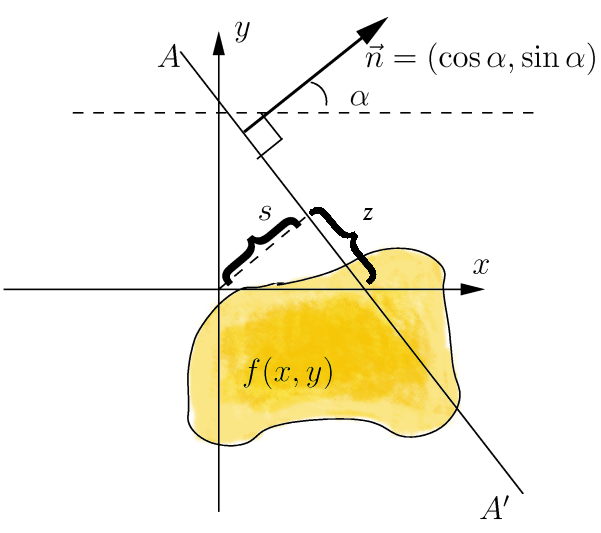
The Radon transform, ${\displaystyle Rf}$, is a function defined on the space of straight lines ${\displaystyle L\subset \mathbb {R} ^{2}}$ by the line integral along each such line as: $${\displaystyle Rf(L)=\int _{L}f(\mathbf {x} )\vert d\mathbf {x} \vert .}$$Concretely, the parametrization of any straight line ${\displaystyle L}$ with respect to arc length ${\displaystyle z}$ can always be written:$${\displaystyle (x(z),y(z))={\Big (}(z\sin \alpha +s\cos \alpha ),(-z\cos \alpha +s\sin \alpha ){\Big )}\,}$$where ${\displaystyle s}$ is the distance of ${\displaystyle L}$ from the origin and ${\displaystyle \alpha }$ is the angle the normal vector to ${\displaystyle L}$ makes with the ${\displaystyle X}$-axis. It follows that the quantities ${\displaystyle (\alpha ,s)}$ can be considered as coordinates on the space of all lines in ${\displaystyle \mathbb {R} ^{2}}$, and the Radon transform can be expressed in these coordinates by: $${\displaystyle {\begin{aligned}Rf(\alpha ,s)&=\int _{-\infty }^{\infty }f(x(z),y(z))\,dz\\&=\int _{-\infty }^{\infty }f{\big (}(z\sin \alpha +s\cos \alpha ),(-z\cos \alpha +s\sin \alpha ){\big )}\,dz.\end{aligned}}}$$More generally, in the ${\displaystyle n}$-dimensional Euclidean space ${\displaystyle \mathbb {R} ^{n}}$, the Radon transform of a function ${\displaystyle f}$ satisfying the regularity conditions is a function ${\displaystyle Rf}$ on the space ${\displaystyle \Sigma _{n}}$ of all hyperplanes in ${\displaystyle \mathbb {R} ^{n}}$. It is defined by:

Shepp Logan phantom

Radon transform

Inverse Radon transform

$${\displaystyle Rf(\xi )=\int _{\xi }f(\mathbf {x} )\,d\sigma (\mathbf {x} ),\quad \forall \xi \in \Sigma _{n}}$$where the integral is taken with respect to the natural hypersurface measure, ${\displaystyle d\sigma }$ (generalizing the ${\displaystyle \vert d\mathbf {x} \vert }$ term from the ${\displaystyle 2}$-dimensional case). Observe that any element of ${\displaystyle \Sigma _{n}}$ is characterized as the solution locus of an equation ${\displaystyle \mathbf {x} \cdot \alpha =s}$, where ${\displaystyle \alpha \in S^{n-1}}$ is a unit vector and ${\displaystyle s\in \mathbb {R} }$. Thus the ${\displaystyle n}$-dimensional Radon transform may be rewritten as a function on ${\displaystyle S^{n-1}\times \mathbb {R} }$ via: $${\displaystyle Rf(\alpha ,s)=\int _{\mathbf {x} \cdot \alpha =s}f(\mathbf {x} )\,d\sigma (\mathbf {x} ).}$$It is also possible to generalize the Radon transform still further by integrating instead over ${\displaystyle k}$-dimensional affine subspaces of ${\displaystyle \mathbb {R} ^{n}}$. The X-ray transform is the most widely used special case of this construction, and is obtained by integrating over straight lines.

The Radon transform is closely related to the Fourier transform. We define the univariate Fourier transform here as: $${\displaystyle {\hat {f}}(\omega )=\int _{-\infty }^{\infty }f(x)e^{-2\pi ix\omega }\,dx.}$$ For a function of a ${\displaystyle 2}$-vector ${\displaystyle \mathbf {x} =(x,y)}$, the univariate Fourier transform is: $${\displaystyle {\hat {f}}(\mathbf {w} )=\iint _{\mathbb {R} ^{2}}f(\mathbf {x} )e^{-2\pi i\mathbf {x} \cdot \mathbf {w} }\,dx\,dy.}$$ For convenience, denote ${\displaystyle {\mathcal {R}}_{\alpha }[f](s)={\mathcal {R}}[f](\alpha ,s)}$. The Fourier slice theorem then states: $${\displaystyle {\widehat {{\mathcal {R}}_{\alpha }[f]}}(\sigma )={\hat {f}}(\sigma \mathbf {n} (\alpha ))}$$ where ${\displaystyle \mathbf {n} (\alpha )=(\cos \alpha ,\sin \alpha ).}$

Thus the two-dimensional Fourier transform of the initial function along a line at the inclination angle ${\displaystyle \alpha }$ is the one variable Fourier transform of the Radon transform (acquired at angle ${\displaystyle \alpha }$) of that function. This fact can be used to compute both the Radon transform and its inverse. The result can be generalized into n dimensions: $${\displaystyle {\hat {f}}(r\alpha )=\int _{\mathbb {R} }{\mathcal {R}}f(\alpha ,s)e^{-2\pi isr}\,ds.}$$

The dual Radon transform is a kind of adjoint to the Radon transform. Beginning with a function g on the space ${\displaystyle \Sigma _{n}}$, the dual Radon transform is the function ${\displaystyle {\mathcal {R}}^{*}g}$ on Rⁿ defined by: $${\displaystyle {\mathcal {R}}^{*}g(\mathbf {x} )=\int _{\mathbf {x} \in \xi }g(\xi )\,d\mu (\xi ).}$$The integral here is taken over the set of all hyperplanes incident with the point ${\displaystyle {\textbf {x}}\in \mathbb {R} ^{n}}$, and the measure ${\displaystyle d\mu }$ is the unique probability measure on the set ${\displaystyle \{\xi |\mathbf {x} \in \xi \}}$ invariant under rotations about the point ${\displaystyle \mathbf {x} }$.

Concretely, for the two-dimensional Radon transform, the dual transform is given by: $${\displaystyle {\mathcal {R}}^{*}g(\mathbf {x} )={\frac {1}{2\pi }}\int _{\alpha =0}^{2\pi }g(\alpha ,\mathbf {n} (\alpha )\cdot \mathbf {x} )\,d\alpha .}$$ In the context of image processing, the dual transform is commonly called back-projection^[4] as it takes a function defined on each line in the plane and 'smears' or projects it back over the line to produce an image.

Let ${\displaystyle \Delta }$ denote the Laplacian on ${\displaystyle \mathbb {R} ^{n}}$ defined by:$${\displaystyle \Delta ={\frac {\partial ^{2}}{\partial x_{1}^{2}}}+\cdots +{\frac {\partial ^{2}}{\partial x_{n}^{2}}}}$$This is a natural rotationally invariant second-order differential operator. On ${\displaystyle \Sigma _{n}}$, the "radial" second derivative ${\displaystyle Lf(\alpha ,s)\equiv {\frac {\partial ^{2}}{\partial s^{2}}}f(\alpha ,s)}$ is also rotationally invariant. The Radon transform and its dual are intertwining operators for these two differential operators in the sense that:^[5] $${\displaystyle {\mathcal {R}}(\Delta f)=L({\mathcal {R}}f),\quad {\mathcal {R}}^{*}(Lg)=\Delta ({\mathcal {R}}^{*}g).}$$In analysing the solutions to the wave equation in multiple spatial dimensions, the intertwining property leads to the translational representation of Lax and Philips.^[6] In imaging^[7] and numerical analysis^[8] this is exploited to reduce multi-dimensional problems into single-dimensional ones, as a dimensional splitting method.

The process of reconstruction produces the image (or function ${\displaystyle f}$ in the previous section) from its projection data. Reconstruction is an inverse problem.

In the two-dimensional case, the most commonly used analytical formula to recover ${\displaystyle f}$ from its Radon transform is the Filtered Back-projection Formula or Radon Inversion Formula^[9]: $${\displaystyle f(\mathbf {x} )=\int _{0}^{\pi }({\mathcal {R}}f(\cdot ,\theta )*h)(\left\langle \mathbf {x} ,\mathbf {n} _{\theta }\right\rangle )\,d\theta }$$where ${\displaystyle h}$ is such that ${\displaystyle {\hat {h}}(k)=|k|}$.^[9] The convolution kernel ${\displaystyle h}$ is referred to as Ramp filter in some literature.

Intuitively, in the filtered back-projection formula, by analogy with differentiation, for which ${\textstyle \left({\widehat {{\frac {d}{dx}}f}}\right)\!(k)=ik{\widehat {f}}(k)}$, we see that the filter performs an operation similar to a derivative. Roughly speaking, then, the filter makes objects more singular. A quantitive statement of the ill-posedness of Radon inversion goes as follows:$${\displaystyle {\widehat {{\mathcal {R}}^{*}{\mathcal {R}}[g]}}(\mathbf {k} )={\frac {1}{\|\mathbf {k} \|}}{\hat {g}}(\mathbf {k} )}$$ where ${\displaystyle {\mathcal {R}}^{*}}$ is the previously defined adjoint to the Radon transform. Thus for ${\displaystyle g(\mathbf {x} )=e^{i\left\langle \mathbf {k} _{0},\mathbf {x} \right\rangle }}$, we have: $${\displaystyle {\mathcal {R}}^{*}{\mathcal {R}}[g](\mathbf {x} )={\frac {1}{\|\mathbf {k_{0}} \|}}e^{i\left\langle \mathbf {k} _{0},\mathbf {x} \right\rangle }}$$ The complex exponential ${\displaystyle e^{i\left\langle \mathbf {k} _{0},\mathbf {x} \right\rangle }}$ is thus an eigenfunction of ${\displaystyle {\mathcal {R}}^{*}{\mathcal {R}}}$ with eigenvalue ${\textstyle {\frac {1}{\|\mathbf {k} _{0}\|}}}$. Thus the singular values of ${\displaystyle {\mathcal {R}}}$ are ${\textstyle {\frac {1}{\sqrt {\|\mathbf {k} \|}}}}$. Since these singular values tend to ${\displaystyle 0}$, ${\displaystyle {\mathcal {R}}^{-1}}$ is unbounded.^[9]

Compared with the Filtered Back-projection method, iterative reconstruction costs large computation time, limiting its practical use. However, due to the ill-posedness of Radon Inversion, the Filtered Back-projection method may be infeasible in the presence of discontinuity or noise. Iterative reconstruction methods (e.g. iterative Sparse Asymptotic Minimum Variance^[10]) could provide metal artefact reduction, noise and dose reduction for the reconstructed result that attract much research interest around the world.

Explicit and computationally efficient inversion formulas for the Radon transform and its dual are available. The Radon transform in ${\displaystyle n}$ dimensions can be inverted by the formula:^[11] $${\displaystyle c_{n}f=(-\Delta )^{(n-1)/2}R^{*}Rf\,}$$where ${\displaystyle c_{n}=(4\pi )^{(n-1)/2}{\frac {\Gamma (n/2)}{\Gamma (1/2)}}}$, and the power of the Laplacian ${\displaystyle (-\Delta )^{(n-1)/2}}$ is defined as a pseudo-differential operator if necessary by the Fourier transform: $${\displaystyle \left[{\mathcal {F}}(-\Delta )^{(n-1)/2}\varphi \right](\xi )=|2\pi \xi |^{n-1}({\mathcal {F}}\varphi )(\xi ).}$$For computational purposes, the power of the Laplacian is commuted with the dual transform ${\displaystyle R^{*}}$ to give:^[12] $${\displaystyle c_{n}f={\begin{cases}R^{*}{\frac {d^{n-1}}{ds^{n-1}}}Rf&n{\text{ odd}}\\R^{*}{\mathcal {H}}_{s}{\frac {d^{n-1}}{ds^{n-1}}}Rf&n{\text{ even}}\end{cases}}}$$where ${\displaystyle {\mathcal {H}}_{s}}$ is the Hilbert transform with respect to the s variable. In two dimensions, the operator ${\displaystyle {\mathcal {H}}_{s}{\frac {d}{ds}}}$ appears in image processing as a ramp filter.^[13] One can prove directly from the Fourier slice theorem and change of variables for integration that for a compactly supported continuous function ${\displaystyle f}$ of two variables: $${\displaystyle f={\frac {1}{2}}R^{*}{\mathcal {H}}_{s}{\frac {d}{ds}}Rf.}$$Thus in an image processing context the original image ${\displaystyle f}$ can be recovered from the 'sinogram' data ${\displaystyle Rf}$ by applying a ramp filter (in the ${\displaystyle s}$ variable) and then back-projecting. As the filtering step can be performed efficiently (for example using digital signal processing techniques) and the back projection step is simply an accumulation of values in the pixels of the image, this results in a highly efficient, and hence widely used, algorithm.

Explicitly, the inversion formula obtained by the latter method is:^[4] $${\displaystyle f(x)={\begin{cases}\displaystyle -\imath 2\pi (2\pi )^{-n}(-1)^{n/2}\int _{S^{n-1}}{\frac {\partial ^{n-1}}{2\partial s^{n-1}}}Rf(\alpha ,\alpha \cdot x)\,d\alpha &n{\text{ odd}}\\\displaystyle (2\pi )^{-n}(-1)^{n/2}\iint _{\mathbb {R} \times S^{n-1}}{\frac {\partial ^{n-1}}{q\partial s^{n-1}}}Rf(\alpha ,\alpha \cdot x+q)\,d\alpha \,dq&n{\text{ even}}\\\end{cases}}}$$The dual transform can also be inverted by an analogous formula: $${\displaystyle c_{n}g=(-L)^{(n-1)/2}R(R^{*}g).\,}$$

In algebraic geometry, a Radon transform (also known as the Brylinski–Radon transform) is constructed as follows.

Write

${\displaystyle \mathbf {P} ^{d}\,{\stackrel {p_{1}}{\gets }}\,H\,{\stackrel {p_{2}}{\to }}\,\mathbf {P} ^{\vee ,d}}$

for the universal hyperplane, i.e., H consists of pairs (x, h) where x is a point in d-dimensional projective space ${\displaystyle \mathbf {P} ^{d}}$ and h is a point in the dual projective space (in other words, x is a line through the origin in (d+1)-dimensional affine space, and h is a hyperplane in that space) such that x is contained in h.

Then the Brylinksi–Radon transform is the functor between appropriate derived categories of étale sheaves

${\displaystyle \operatorname {Rad} :=Rp_{2,*}p_{1}^{*}:D(\mathbf {P} ^{d})\to D(\mathbf {P} ^{\vee ,d}).}$

The main theorem about this transform is that this transform induces an equivalence of the categories of perverse sheaves on the projective space and its dual projective space, up to constant sheaves.^[14]

• Periodogram
• Matched filter
• Deconvolution
• X-ray transform
• Funk transform
• The Hough transform, when written in a continuous form, is very similar, if not equivalent, to the Radon transform.^[15]
• Cauchy–Crofton theorem is a closely related formula for computing the length of curves in space.
• Fast Fourier transform

References

[edit]- Kiehl, Reinhardt; Weissauer, Rainer (2001), Weil conjectures, perverse sheaves and l'adic Fourier transform, Springer, doi:10.1007/978-3-662-04576-3, ISBN 3-540-41457-6, MR 1855066
- Radon, Johann (1917), "Über die Bestimmung von Funktionen durch ihre Integralwerte längs gewisser Mannigfaltigkeiten", Berichte über die Verhandlungen der Königlich-Sächsischen Akademie der Wissenschaften zu Leipzig, Mathematisch-Physische Klasse [Reports on the Proceedings of the Royal Saxonian Academy of Sciences at Leipzig, Mathematical and Physical Section] (69), Leipzig: Teubner: 262–277;
Translation: Radon, J. (December 1986), "On the determination of functions from their integral values along certain manifolds", IEEE Transactions on Medical Imaging, 5 (4), translated by Parks, P.C.: 170–176, doi:10.1109/TMI.1986.4307775, PMID 18244009, S2CID 26553287. - Roerdink, J.B.T.M. (2001) [1994], "Tomography", Encyclopedia of Mathematics, EMS Press.
- Helgason, Sigurdur (1984), Groups and Geometric Analysis: Integral Geometry, Invariant Differential Operators, and Spherical Functions, Academic Press, ISBN 0-12-338301-3.
- Candès, Emmanuel (February 9, 2021a). "Applied Fourier Analysis and Elements of Modern Signal Processing – Lecture 9" (PDF).
- Candès, Emmanuel (February 11, 2021b). "Applied Fourier Analysis and Elements of Modern Signal Processing – Lecture 10" (PDF).
- Nygren, Anders J. (1997). "Filtered Back Projection". Tomographic Reconstruction of SPECT Data.
- van Ginkel, M.; Hendricks, C.L. Luengo; van Vliet, L.J. (2004). "A short introduction to the Radon and Hough transforms and how they relate to each other" (PDF). Archived (PDF) from the original on 2016-07-29.
Further reading
[edit]- Lokenath Debnath; Dambaru Bhatta (19 April 2016). Integral Transforms and Their Applications. CRC Press. ISBN 978-1-4200-1091-6.
- Deans, Stanley R. (1983), The Radon Transform and Some of Its Applications, New York: John Wiley & Sons
- Helgason, Sigurdur (2008), Geometric analysis on symmetric spaces, Mathematical Surveys and Monographs, vol. 39 (2nd ed.), Providence, R.I.: American Mathematical Society, doi:10.1090/surv/039, ISBN 978-0-8218-4530-1, MR 2463854
- Herman, Gabor T. (2009), Fundamentals of Computerized Tomography: Image Reconstruction from Projections (2nd ed.), Springer, ISBN 978-1-85233-617-2
- Minlos, R.A. (2001) [1994], "Radon transform", Encyclopedia of Mathematics, EMS Press
- Natterer, Frank (June 2001), The Mathematics of Computerized Tomography, Classics in Applied Mathematics, vol. 32, Society for Industrial and Applied Mathematics, ISBN 0-89871-493-1
- Natterer, Frank; Wübbeling, Frank (2001), Mathematical Methods in Image Reconstruction, Society for Industrial and Applied Mathematics, Bibcode:2001mmir.book.....N, ISBN 0-89871-472-9
External links
[edit]- Weisstein, Eric W. "Radon Transform". MathWorld.
- Analytical projection (the Radon transform) (video). Part of the "Computed Tomography and the ASTRA Toolbox" course. University of Antwerp. September 10, 2015.