In materials science, a Bingham plastic is a viscoplastic material that behaves as a rigid body at low stresses but flows as a viscous fluid at high stress. It is named after Eugene C. Bingham who proposed its mathematical form in 1916.

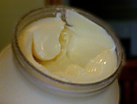
It is used as a common mathematical model of mud flow in drilling engineering, and in the handling of slurries. A common example is toothpaste, which will not be extruded until a certain pressure is applied to the tube. It is then pushed out as a relatively coherent plug.

Figure 1 shows a graph of the behaviour of an ordinary viscous (or Newtonian) fluid in red, for example in a pipe. If the pressure at one end of a pipe is increased this produces a stress on the fluid tending to make it move (called the shear stress) and the volumetric flow rate increases proportionally. However, for a Bingham Plastic fluid (in blue), stress can be applied but it will not flow until a certain value, the yield stress, is reached. Beyond this point the flow rate increases steadily with increasing shear stress. This is roughly the way in which Bingham presented his observation, in an experimental study of paints. These properties allow a Bingham plastic to have a textured surface with peaks and ridges instead of a featureless surface like a Newtonian fluid.

Figure 2 shows the way in which it is normally presented currently. The graph shows shear stress on the vertical axis and shear rate on the horizontal one. (Volumetric flow rate depends on the size of the pipe, shear rate is a measure of how the velocity changes with distance. It is proportional to flow rate, but does not depend on pipe size.) As before, the Newtonian fluid flows and gives a shear rate for any finite value of shear stress. However, the Bingham plastic again does not exhibit any shear rate (no flow and thus no velocity) until a certain stress is achieved. For the Newtonian fluid the slope of this line is the viscosity, which is the only parameter needed to describe its flow. By contrast, the Bingham plastic requires two parameters, the yield stress and the slope of the line, known as the plastic viscosity.

The physical reason for this behaviour is that the liquid contains particles (such as clay) or large molecules (such as polymers) which have some kind of interaction, creating a weak solid structure, formerly known as a false body, and a certain amount of stress is required to break this structure. Once the structure has been broken, the particles move with the liquid under viscous forces. If the stress is removed, the particles associate again.

The material is an elastic solid for shear stress ${\displaystyle \tau }$, less than a critical value ${\displaystyle \tau _{0}}$. Once the critical shear stress (or "yield stress") is exceeded, the material flows in such a way that the shear rate, ∂u/∂y (as defined in the article on viscosity), is directly proportional to the amount by which the applied shear stress exceeds the yield stress:

In fluid flow, it is a common problem to calculate the pressure drop in an established piping network. Once the friction factor, f, is known, it becomes easier to handle different pipe-flow problems, viz. calculating the pressure drop for evaluating pumping costs or to find the flow-rate in a piping network for a given pressure drop. It is usually extremely difficult to arrive at exact analytical solution to calculate the friction factor associated with flow of non-Newtonian fluids and therefore explicit approximations are used to calculate it. Once the friction factor has been calculated the pressure drop can be easily determined for a given flow by the Darcy–Weisbach equation:

where: