

Power law
View on Wikipedia
In statistics, a power law is a functional relationship between two quantities, where a relative change in one quantity results in a relative change in the other quantity proportional to the change raised to a constant exponent: one quantity varies as a power of another. The change is independent of the initial size of those quantities.
For instance, the area of a square has a power law relationship with the length of its side, since if the length is doubled, the area is multiplied by 22, while if the length is tripled, the area is multiplied by 32, and so on.[1]
Empirical examples
[edit]The distributions of a wide variety of physical, biological, and human-made phenomena approximately follow a power law over a wide range of magnitudes: these include the sizes of craters on the moon and of solar flares,[2] cloud sizes,[3] the foraging pattern of various species,[4] the sizes of activity patterns of neuronal populations,[5] the frequencies of words in most languages, frequencies of family names, the species richness in clades of organisms,[6] the sizes of power outages, volcanic eruptions,[7] human judgments of stimulus intensity[8][9] and many other quantities.[10] Empirical distributions can only fit a power law for a limited range of values, because a pure power law would allow for arbitrarily large or small values. Acoustic attenuation follows frequency power-laws within wide frequency bands for many complex media. Allometric scaling laws for relationships between biological variables are among the best known power-law functions in nature.
Properties
[edit]Statistical incompleteness
[edit]The power-law model does not obey the treasured paradigm of statistical completeness. Especially probability bounds, the suspected cause of typical bending and/or flattening phenomena in the high- and low-frequency graphical segments, are parametrically absent in the standard model.[11]
Scale invariance
[edit]One attribute of power laws is their scale invariance. Given a relation , scaling the argument by a constant factor causes only a proportionate scaling of the function itself. That is,
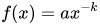



where denotes direct proportionality. That is, scaling by a constant simply multiplies the original power-law relation by the constant . Thus, it follows that all power laws with a particular scaling exponent are equivalent up to constant factors, since each is simply a scaled version of the others. This behavior is what produces the linear relationship when logarithms are taken of both and , and the straight-line on the log–log plot is often called the signature of a power law. With real data, such straightness is a necessary, but not sufficient, condition for the data following a power-law relation. In fact, there are many ways to generate finite amounts of data that mimic this signature behavior, but, in their asymptotic limit, are not true power laws.[citation needed] Thus, accurately fitting and validating power-law models is an active area of research in statistics; see below.


Lack of well-defined average value
[edit]A power-law has a well-defined mean over only if , and it has a finite variance only if ; most identified power laws in nature have exponents such that the mean is well-defined but the variance is not, implying they are capable of black swan behavior.[2] This can be seen in the following thought experiment:[12] imagine a room with your friends and estimate the average monthly income in the room. Now imagine the world's richest person entering the room, with a monthly income of about 1 billion US$. What happens to the average income in the room? Income is distributed according to a power-law known as the Pareto distribution (for example, the net worth of Americans is distributed according to a power law with an exponent of 2).


On the one hand, this makes it incorrect to apply traditional statistics that are based on variance and standard deviation (such as regression analysis).[13] On the other hand, this also allows for cost-efficient interventions.[12] For example, given that car exhaust is distributed according to a power-law among cars (very few cars contribute to most contamination) it would be sufficient to eliminate those very few cars from the road to reduce total exhaust substantially.[14]
The median does exist, however: for a power law x –k, with exponent , it takes the value 21/(k – 1)xmin, where xmin is the minimum value for which the power law holds.[2]

Universality
[edit]The equivalence of power laws with a particular scaling exponent can have a deeper origin in the dynamical processes that generate the power-law relation. In physics, for example, phase transitions in thermodynamic systems are associated with the emergence of power-law distributions of certain quantities, whose exponents are referred to as the critical exponents of the system. Diverse systems with the same critical exponents—that is, which display identical scaling behaviour as they approach criticality—can be shown, via renormalization group theory, to share the same fundamental dynamics. For instance, the behavior of water and CO2 at their boiling points fall in the same universality class because they have identical critical exponents.[citation needed][clarification needed] In fact, almost all material phase transitions are described by a small set of universality classes. Similar observations have been made, though not as comprehensively, for various self-organized critical systems, where the critical point of the system is an attractor. Formally, this sharing of dynamics is referred to as universality, and systems with precisely the same critical exponents are said to belong to the same universality class.
Power-law functions
[edit]Scientific interest in power-law relations stems partly from the ease with which certain general classes of mechanisms generate them.[15] The demonstration of a power-law relation in some data can point to specific kinds of mechanisms that might underlie the natural phenomenon in question, and can indicate a deep connection with other, seemingly unrelated systems;[16] see also universality above. The ubiquity of power-law relations in physics is partly due to dimensional constraints, while in complex systems, power laws are often thought to be signatures of hierarchy or of specific stochastic processes. A few notable examples of power laws are Pareto's law of income distribution, structural self-similarity of fractals, scaling laws in biological systems, and scaling laws in cities. Research on the origins of power-law relations, and efforts to observe and validate them in the real world, is an active topic of research in many fields of science, including physics, computer science, linguistics, geophysics, neuroscience, systematics, sociology, economics and more.
However, much of the recent interest in power laws comes from the study of probability distributions: The distributions of a wide variety of quantities seem to follow the power-law form, at least in their upper tail (large events). The behavior of these large events connects these quantities to the study of theory of large deviations (also called extreme value theory), which considers the frequency of extremely rare events like stock market crashes and large natural disasters. It is primarily in the study of statistical distributions that the name "power law" is used.
In empirical contexts, an approximation to a power-law often includes a deviation term , which can represent uncertainty in the observed values (perhaps measurement or sampling errors) or provide a simple way for observations to deviate from the power-law function (perhaps for stochastic reasons):


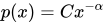
Mathematically, a strict power law cannot be a probability distribution, but a distribution that is a truncated power function is possible: for where the exponent (Greek letter alpha, not to be confused with scaling factor used above) is greater than 1 (otherwise the tail has infinite area), the minimum value is needed otherwise the distribution has infinite area as x approaches 0, and the constant C is a scaling factor to ensure that the total area is 1, as required by a probability distribution. More often one uses an asymptotic power law – one that is only true in the limit; see power-law probability distributions below for details. Typically the exponent falls in the range , though not always.[10]


Examples
[edit]More than a hundred power-law distributions have been identified in physics (e.g. sandpile avalanches), biology (e.g. species extinction and body mass), and the social sciences (e.g. city sizes and income).[17] Among them are:
Artificial Intelligence
[edit]Astronomy
[edit]- Kepler's third law
- The initial mass function of stars
- The differential energy spectrum of cosmic-ray nuclei
- The M–sigma relation
- Solar flares
Biology
[edit]- Kleiber's law relating animal metabolism to size, and allometric laws in general
- The two-thirds power law, relating speed to curvature in the human motor system.[18]
- The Taylor's law relating mean population size and variance of populations sizes in ecology
- Neuronal avalanches[5]
- The species richness (number of species) in clades of freshwater fishes[19]
- The Harlow Knapp effect, where a subset of the kinases found in the human body compose a majority of published research[20]
- The size of forest patches globally follows a power law [21]
- The species–area relationship relating the number of species found in an area as a function of the size of the area
Chemistry
[edit]Climate science
[edit]- Sizes of cloud areas and perimeters, as viewed from space[3]
- The size of rain-shower cells[22]
- Energy dissipation in cyclones[23]
- Diameters of dust devils on Earth and Mars [24]
General science
[edit]- Highly optimized tolerance
- Proposed form of experience curve effects
- Pink noise
- The law of stream numbers, and the law of stream lengths (Horton's laws describing river systems)[25]
- Populations of cities (Gibrat's law)[26]
- Bibliograms, and frequencies of words in a text (Zipf's law)[27]
- 90–9–1 principle on wikis (also referred to as the 1% rule)[28][29]
- Richardson's Law for the severity of violent conflicts (wars and terrorism)[30][31]
- The relationship between a CPU's cache size and the number of cache misses follows the power law of cache misses.
- The spectral density of the weight matrices of deep neural networks[32]
- Associated with exponential growth:
- Tails in statistical distributions for exponential growth processes with random observation (or killing)[33]
- Progress through exponential growth and exponential diffusion of innovations[34]
Economics
[edit]- Population sizes of cities in a region or urban network, Zipf's law.
- Distribution of artists by the average price of their artworks.[35]
- Income distribution in a market economy.
- Distribution of degrees in banking networks.[36]
- Firm-size distributions.[37]
- Scaling laws of socio-economic quantities with respect to population size (see urban scaling).[38][39]
Finance
[edit]- Returns for high-risk venture capital investments[40]
- The mean absolute change of the logarithmic mid-prices[41]
- Large price changes, volatility, and transaction volume on stock exchanges[42]
- Average waiting time of a directional change[43]
- Average waiting time of an overshoot
Mathematics
[edit]- Fractals
- Pareto distribution and the Pareto principle also called the "80–20 rule"
- Zipf's law in corpus analysis and population distributions amongst others, where frequency of an item or event is inversely proportional to its frequency rank (i.e. the second most frequent item/event occurs half as often as the most frequent item, the third most frequent item/event occurs one third as often as the most frequent item, and so on).
- Zeta distribution (discrete)
- Yule–Simon distribution (discrete)
- Student's t-distribution (continuous), of which the Cauchy distribution is a special case
- Lotka's law
- The scale-free network model
Physics
[edit]- The Angstrom exponent in aerosol optics
- The frequency-dependency of acoustic attenuation in complex media
- The Stefan–Boltzmann law
- The input-voltage–output-current curves of field-effect transistors and vacuum tubes approximate a square-law relationship, a factor in "tube sound".
- Square–cube law (ratio of surface area to volume)
- A 3/2-power law can be found in the plate characteristic curves of triodes.
- The inverse-square laws of Newtonian gravity and electrostatics, as evidenced by the gravitational potential and Electrostatic potential, respectively.
- Self-organized criticality with a critical point as an attractor
- Model of van der Waals force
- Force and potential in simple harmonic motion
- Gamma correction relating light intensity with voltage
- Behaviour near second-order phase transitions involving critical exponents
- The safe operating area relating to maximum simultaneous current and voltage in power semiconductors.
- Supercritical state of matter and supercritical fluids, such as supercritical exponents of heat capacity and viscosity.[44]
- The Curie–von Schweidler law in dielectric responses to step DC voltage input.
- The damping force over speed relation in antiseismic dampers calculus
- Folded solvent-exposed surface areas of centered amino acids in protein structure segments[45]
Political Science
[edit]- Cube root law of assembly sizes
Psychology
[edit]- Stevens's power law of psychophysics (challenged with demonstrations that it may be logarithmic[46][47])
- The power law of forgetting[48]
Variants
[edit]Broken power law
[edit]
A broken power law is a piecewise function, consisting of two or more power laws, combined with a threshold. For example, with two power laws:[49]
for ,


Smoothly broken power law
[edit]The pieces of a broken power law can be smoothly spliced together to construct a smoothly broken power law.
There are different possible ways to splice together power laws. One example is the following:[50]where .


When the function is plotted as a log-log plot with horizontal axis being and vertical axis being , the plot is composed of linear segments with slopes , separated at , smoothly spliced together. The size of determines the sharpness of splicing between segments .






Power law with exponential cutoff
[edit]A power law with an exponential cutoff is simply a power law multiplied by an exponential function:[10]

Curved power law
[edit]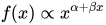
Power-law probability distributions
[edit]In a looser sense, a power-law probability distribution is a distribution whose density function (or mass function in the discrete case) has the form, for large values of ,[52]

where , and is a slowly varying function, which is any function that satisfies for any positive factor . This property of follows directly from the requirement that be asymptotically scale invariant; thus, the form of only controls the shape and finite extent of the lower tail. For instance, if is the constant function, then we have a power law that holds for all values of . In many cases, it is convenient to assume a lower bound from which the law holds. Combining these two cases, and where is a continuous variable, the power law has the form of the Pareto distribution


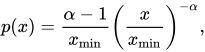
where the pre-factor to is the normalizing constant. We can now consider several properties of this distribution. For instance, its moments are given by


which is only well defined for . That is, all moments diverge: when , the average and all higher-order moments are infinite; when , the mean exists, but the variance and higher-order moments are infinite, etc. For finite-size samples drawn from such distribution, this behavior implies that the central moment estimators (like the mean and the variance) for diverging moments will never converge – as more data is accumulated, they continue to grow. These power-law probability distributions are also called Pareto-type distributions, distributions with Pareto tails, or distributions with regularly varying tails.


A modification, which does not satisfy the general form above, with an exponential cutoff,[10] is

In this distribution, the exponential decay term eventually overwhelms the power-law behavior at very large values of . This distribution does not scale[further explanation needed] and is thus not asymptotically as a power law; however, it does approximately scale over a finite region before the cutoff. The pure form above is a subset of this family, with . This distribution is a common alternative to the asymptotic power-law distribution because it naturally captures finite-size effects.


The Tweedie distributions are a family of statistical models characterized by closure under additive and reproductive convolution as well as under scale transformation. Consequently, these models all express a power-law relationship between the variance and the mean. These models have a fundamental role as foci of mathematical convergence similar to the role that the normal distribution has as a focus in the central limit theorem. This convergence effect explains why the variance-to-mean power law manifests so widely in natural processes, as with Taylor's law in ecology and with fluctuation scaling[53] in physics. It can also be shown that this variance-to-mean power law, when demonstrated by the method of expanding bins, implies the presence of 1/f noise and that 1/f noise can arise as a consequence of this Tweedie convergence effect.[54]
Graphical methods for identification
[edit]Although more sophisticated and robust methods have been proposed, the most frequently used graphical methods of identifying power-law probability distributions using random samples are Pareto quantile-quantile plots (or Pareto Q–Q plots),[citation needed] mean residual life plots[55][56] and log–log plots. Another, more robust graphical method uses bundles of residual quantile functions.[57] (Please keep in mind that power-law distributions are also called Pareto-type distributions.) It is assumed here that a random sample is obtained from a probability distribution, and that we want to know if the tail of the distribution follows a power law (in other words, we want to know if the distribution has a "Pareto tail"). Here, the random sample is called "the data".
Pareto Q–Q plots
[edit]Pareto Q–Q plots compare the quantiles of the log-transformed data to the corresponding quantiles of an exponential distribution with mean 1 (or to the quantiles of a standard Pareto distribution) by plotting the former versus the latter. If the resultant scatterplot suggests that the plotted points asymptotically converge to a straight line, then a power-law distribution should be suspected. A limitation of Pareto Q–Q plots is that they behave poorly when the tail index (also called Pareto index) is close to 0, because Pareto Q–Q plots are not designed to identify distributions with slowly varying tails.[57]
Mean residual life plots
[edit]On the other hand, in its version for identifying power-law probability distributions, the mean residual life plot consists of first log-transforming the data, and then plotting the average of those log-transformed data that are higher than the i-th order statistic versus the i-th order statistic, for i = 1, ..., n, where n is the size of the random sample. If the resultant scatterplot suggests that the plotted points tend to stabilize about a horizontal straight line, then a power-law distribution should be suspected. Since the mean residual life plot is very sensitive to outliers (it is not robust), it usually produces plots that are difficult to interpret; for this reason, such plots are usually called Hill horror plots.[58]
Log-log plots
[edit]
Log–log plots are an alternative way of graphically examining the tail of a distribution using a random sample. Taking the logarithm of a power law of the form results in:[59]


which forms a straight line with slope on a log-log scale. Caution has to be exercised however as a log–log plot is necessary but insufficient evidence for a power law relationship, as many non power-law distributions will appear as straight lines on a log–log plot.[10][60] This method consists of plotting the logarithm of an estimator of the probability that a particular number of the distribution occurs versus the logarithm of that particular number. Usually, this estimator is the proportion of times that the number occurs in the data set. If the points in the plot tend to converge to a straight line for large numbers in the x axis, then the researcher concludes that the distribution has a power-law tail. Examples of the application of these types of plot have been published.[61] A disadvantage of these plots is that, in order for them to provide reliable results, they require huge amounts of data. In addition, they are appropriate only for discrete (or grouped) data.

Bundle plots
[edit]Another graphical method for the identification of power-law probability distributions using random samples has been proposed.[57] This methodology consists of plotting a bundle for the log-transformed sample. Originally proposed as a tool to explore the existence of moments and the moment generation function using random samples, the bundle methodology is based on residual quantile functions (RQFs), also called residual percentile functions,[62][63][64][65][66][67][68] which provide a full characterization of the tail behavior of many well-known probability distributions, including power-law distributions, distributions with other types of heavy tails, and even non-heavy-tailed distributions. Bundle plots do not have the disadvantages of Pareto Q–Q plots, mean residual life plots and log–log plots mentioned above (they are robust to outliers, allow visually identifying power laws with small values of , and do not demand the collection of much data).[citation needed] In addition, other types of tail behavior can be identified using bundle plots.
Plotting power-law distributions
[edit]In general, power-law distributions are plotted on doubly logarithmic axes, which emphasizes the upper tail region. The most convenient way to do this is via the (complementary) cumulative distribution (ccdf) that is, the survival function, ,


The cdf is also a power-law function, but with a smaller scaling exponent. For data, an equivalent form of the cdf is the rank-frequency approach, in which we first sort the observed values in ascending order, and plot them against the vector .

![{\displaystyle \left[1,{\frac {n-1}{n}},{\frac {n-2}{n}},\dots ,{\frac {1}{n}}\right]}](https://wikimedia.org/api/rest_v1/media/math/render/svg/c0175b6d7f7d253c98fdd81995d23a3996605f7b)
Although it can be convenient to log-bin the data, or otherwise smooth the probability density (mass) function directly, these methods introduce an implicit bias in the representation of the data, and thus should be avoided.[10][69] The survival function, on the other hand, is more robust to (but not without) such biases in the data and preserves the linear signature on doubly logarithmic axes. Though a survival function representation is favored over that of the pdf while fitting a power law to the data with the linear least square method, it is not devoid of mathematical inaccuracy. Thus, while estimating exponents of a power law distribution, maximum likelihood estimator is recommended.
Estimating the exponent from empirical data
[edit]There are many ways of estimating the value of the scaling exponent for a power-law tail, however not all of them yield unbiased and consistent answers. Some of the most reliable techniques are often based on the method of maximum likelihood. Alternative methods are often based on making a linear regression on either the log–log probability, the log–log cumulative distribution function, or on log-binned data, but these approaches should be avoided as they can all lead to highly biased estimates of the scaling exponent.[10]
Maximum likelihood
[edit]For real-valued, independent and identically distributed data, we fit a power-law distribution of the form
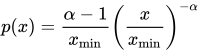
to the data , where the coefficient is included to ensure that the distribution is normalized. Given a choice for , the log likelihood function becomes:


The maximum of this likelihood is found by differentiating with respect to parameter , setting the result equal to zero. Upon rearrangement, this yields the estimator equation:
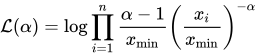
![{\displaystyle {\hat {\alpha }}=1+n\left[\sum _{i=1}^{n}\ln {\frac {x_{i}}{x_{\min }}}\right]^{-1}}](https://wikimedia.org/api/rest_v1/media/math/render/svg/f7eefef62e3201d54661e22ee7ebf59b2dddf3fb)
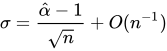
where are the data points .[2][70] This estimator exhibits a small finite sample-size bias of order , which is small when n > 100. Further, the standard error of the estimate is . This estimator is equivalent to the popular[citation needed] Hill estimator from quantitative finance and extreme value theory.[citation needed]


For a set of n integer-valued data points , again where each , the maximum likelihood exponent is the solution to the transcendental equation
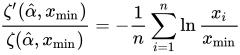
where is the incomplete zeta function. The uncertainty in this estimate follows the same formula as for the continuous equation. However, the two equations for are not equivalent, and the continuous version should not be applied to discrete data, nor vice versa.


Further, both of these estimators require the choice of . For functions with a non-trivial function, choosing too small produces a significant bias in , while choosing it too large increases the uncertainty in , and reduces the statistical power of our model. In general, the best choice of depends strongly on the particular form of the lower tail, represented by above.
More about these methods, and the conditions under which they can be used, can be found in .[10] Further, this comprehensive review article provides usable code (Matlab, Python, R and C++) for estimation and testing routines for power-law distributions.
Kolmogorov–Smirnov estimation
[edit]Another method for the estimation of the power-law exponent, which does not assume independent and identically distributed (iid) data, uses the minimization of the Kolmogorov–Smirnov statistic, , between the cumulative distribution functions of the data and the power law:


with

where and denote the cdfs of the data and the power law with exponent , respectively. As this method does not assume iid data, it provides an alternative way to determine the power-law exponent for data sets in which the temporal correlation can not be ignored.[5]


Validating power laws
[edit]Although power-law relations are attractive for many theoretical reasons, demonstrating that data does indeed follow a power-law relation requires more than simply fitting a particular model to the data.[34] This is important for understanding the mechanism that gives rise to the distribution: superficially similar distributions may arise for significantly different reasons, and different models yield different predictions, such as extrapolation.
For example, log-normal distributions are often mistaken for power-law distributions:[71]. When you take the log of its probability density function, the log-normal distribution has terms that are constant, log, and log-squared. When the mean is small and variance is large, the constant in front of the log-squared term is very small. In that case, for most of the distribution, it will be linear on a log-log plot. It is only for extreme values that the log-squared term asserts itself and shows that it is not a power-law.
For example, Gibrat's law about proportional growth processes produce distributions that are lognormal, although their log–log plots look linear over a limited range. An explanation of this is that although the logarithm of the lognormal density function is quadratic in log(x), yielding a "bowed" shape in a log–log plot, if the quadratic term is small relative to the linear term then the result can appear almost linear, and the lognormal behavior is only visible when the quadratic term dominates, which may require significantly more data. Therefore, a log–log plot that is slightly "bowed" downwards can reflect a log-normal distribution – not a power law.
In general, many alternative functional forms can appear to follow a power-law form for some extent.[72] Stumpf & Porter (2012) proposed plotting the empirical cumulative distribution function in the log-log domain and claimed that a candidate power-law should cover at least two orders of magnitude.[73] Also, researchers usually have to face the problem of deciding whether or not a real-world probability distribution follows a power law. As a solution to this problem, Diaz[57] proposed a graphical methodology based on random samples that allow visually discerning between different types of tail behavior. This methodology uses bundles of residual quantile functions, also called percentile residual life functions, which characterize many different types of distribution tails, including both heavy and non-heavy tails. However, Stumpf & Porter (2012) claimed the need for both a statistical and a theoretical background in order to support a power-law in the underlying mechanism driving the data generating process.[73]
One method to validate a power-law relation tests many orthogonal predictions of a particular generative mechanism against data. Simply fitting a power-law relation to a particular kind of data is not considered a rational approach. As such, the validation of power-law claims remains a very active field of research in many areas of modern science.[10]
See also
[edit]References
[edit]Notes
- ^ Yaneer Bar-Yam. "Concepts: Power Law". New England Complex Systems Institute. Retrieved 18 August 2015.
- ^ a b c d Newman, M. E. J. (2005). "Power laws, Pareto distributions and Zipf's law". Contemporary Physics. 46 (5): 323–351. arXiv:cond-mat/0412004. Bibcode:2005ConPh..46..323N. doi:10.1080/00107510500052444. S2CID 202719165.
- ^ a b DeWitt, Thomas D.; Garrett, Timothy J.; Rees, Karlie N.; Bois, Corey; Krueger, Steven K.; Ferlay, Nicolas (2024-01-05). "Climatologically invariant scale invariance seen in distributions of cloud horizontal sizes". Atmospheric Chemistry and Physics. 24 (1): 109–122. Bibcode:2024ACP....24..109D. doi:10.5194/acp-24-109-2024. ISSN 1680-7316.
- ^ Humphries NE, Queiroz N, Dyer JR, Pade NG, Musyl MK, Schaefer KM, Fuller DW, Brunnschweiler JM, Doyle TK, Houghton JD, Hays GC, Jones CS, Noble LR, Wearmouth VJ, Southall EJ, Sims DW (2010). "Environmental context explains Lévy and Brownian movement patterns of marine predators" (PDF). Nature. 465 (7301): 1066–1069. Bibcode:2010Natur.465.1066H. doi:10.1038/nature09116. PMID 20531470. S2CID 4316766.
- ^ a b c Klaus A, Yu S, Plenz D (2011). Zochowski M (ed.). "Statistical Analyses Support Power Law Distributions Found in Neuronal Avalanches". PLOS ONE. 6 (5). e19779. Bibcode:2011PLoSO...619779K. doi:10.1371/journal.pone.0019779. PMC 3102672. PMID 21720544.
- ^ Albert & Reis 2011, p. [page needed].
- ^ Cannavò, Flavio; Nunnari, Giuseppe (2016-03-01). "On a Possible Unified Scaling Law for Volcanic Eruption Durations". Scientific Reports. 6 22289. Bibcode:2016NatSR...622289C. doi:10.1038/srep22289. ISSN 2045-2322. PMC 4772095. PMID 26926425.
- ^ Stevens, S. S. (1957). "On the psychophysical law". Psychological Review. 64 (3): 153–181. doi:10.1037/h0046162. PMID 13441853.
- ^ Staddon, J. E. R. (1978). "Theory of behavioral power functions". Psychological Review. 85 (4): 305–320. doi:10.1037/0033-295x.85.4.305. hdl:10161/6003.
- ^ a b c d e f g h i Clauset, Shalizi & Newman 2009.
- ^ Van Droogenbroeck, Frans J., 'Completion of the standard power-law model by including upper and lower probability bounds' (2023).
- ^ a b "9na CEPAL Charlas Sobre Sistemas Complejos Sociales (CCSSCS): Leyes de potencias". YouTube. 31 December 2013.
- ^ Taleb, Nassim Nicholas; Bar-Yam, Yaneer; Cirillo, Pasquale (2020-10-20). "On single point forecasts for fat-tailed variables". International Journal of Forecasting. 38 (2): 413–422. doi:10.1016/j.ijforecast.2020.08.008. ISSN 0169-2070. PMC 7572356. PMID 33100449. S2CID 220919883.
- ^ Malcolm Gladwell (February 13, 2006). "Million-Dollar Murray". Archived from the original on 2015-03-18. Retrieved 2015-06-14.
- ^ Sornette 2006.
- ^ Simon 1955.
- ^ Andriani, P.; McKelvey, B. (2007). "Beyond Gaussian averages: redirecting international business and management research toward extreme events and power laws". Journal of International Business Studies. 38 (7): 1212–1230. doi:10.1057/palgrave.jibs.8400324. S2CID 512642.
- ^ Lacquaniti, Francesco; Terzuolo, Carlo; Viviani, Paolo (1983). "The law relating the kinematic and figural aspects of drawing movements". Acta Psychologica. 54 (1–3): 115–130. doi:10.1016/0001-6918(83)90027-6. PMID 6666647. S2CID 5144040.
- ^ Albert, J. S.; Bart, H. J.; Reis, R. E. "Species richness & cladal diversity". In Albert & Reis (2011), pp. 89–104.
- ^ Yu, Frank H.; Willson, Timothy; Frye, Stephen; Edwards, Aled; Bader, Gary D.; Isserlin, Ruth (2011-02-02). "The human genome and drug discovery after a decade. Roads (still) not taken". Nature. 470 (7333): 163–165. arXiv:1102.0448v2. Bibcode:2011Natur.470..163E. doi:10.1038/470163a. PMID 21307913. S2CID 4429387.
- ^ Saravia, Leonardo A.; Doyle, Santiago R.; Bond-Lamberty, Ben (2018-12-10). "Power laws and critical fragmentation in global forests". Scientific Reports. 8 (1): 17766. Bibcode:2018NatSR...817766S. doi:10.1038/s41598-018-36120-w. ISSN 2045-2322. PMC 6288094. PMID 30532065.
- ^ Machado L, Rossow, WB (1993). "Structural characteristics and radial properties of tropical cloud clusters". Monthly Weather Review. 121 (12): 3234–3260. doi:10.1175/1520-0493(1993)121<3234:scarpo>2.0.co;2.
- ^ Corral, A, Osso, A, Llebot, JE (2010). "Scaling of tropical cyclone dissipation". Nature Physics. 6 (9): 693–696. arXiv:0910.0054. Bibcode:2010NatPh...6..693C. doi:10.1038/nphys1725. S2CID 67754747.
- ^ Lorenz RD (2009). "Power Law of Dust Devil Diameters on Earth and Mars". Icarus. 203 (2): 683–684. Bibcode:2009Icar..203..683L. doi:10.1016/j.icarus.2009.06.029.
- ^ "Horton's Laws – Example". www.engr.colostate.edu. Retrieved 2018-09-30.
- ^ Sutton, J. (1997), "Gibrat's Legacy", Journal of Economic Literature XXXV, 40–59.
- ^ Li, W. (November 1999). "Random texts exhibit Zipf's-law-like word frequency distribution". IEEE Transactions on Information Theory. 38 (6): 1842–1845. doi:10.1109/18.165464. ISSN 0018-9448.
- ^ Curtis, Vickie (2018-04-20). Online Citizen Science and the Widening of Academia: Distributed Engagement with Research and Knowledge Production. Springer. ISBN 978-3-319-77664-4.
- ^ Croteau, David; Hoynes, William (2013-11-06). Media/Society: Industries, Images, and Audiences. SAGE Publications. ISBN 978-1-4833-2355-8.
- ^ Lewis Fry Richardson (1950). The Statistics of Deadly Quarrels.
- ^ Berreby, David (July 31, 2014). "Cloudy With a Chance of War". Nautilus Magazine. Retrieved October 22, 2020.
- ^ Martin, Charles H.; Mahoney, Michael W. (2018-10-02). "Implicit Self-Regularization in Deep Neural Networks: Evidence from Random Matrix Theory and Implications for Learning". arXiv:1810.01075 [cs.LG].
- ^ Reed, W. J.; Hughes, B. D. (2002). "From gene families and genera to incomes and internet file sizes: Why power laws are so common in nature" (PDF). Phys Rev E. 66 (6) 067103. Bibcode:2002PhRvE..66f7103R. doi:10.1103/physreve.66.067103. PMID 12513446.
- ^ a b Hilbert, Martin (2013). "Scale-free power-laws as interaction between progress and diffusion". Complexity (Submitted manuscript). 19 (4): 56–65. Bibcode:2014Cmplx..19d..56H. doi:10.1002/cplx.21485.
- ^ Etro, F.; Stepanova, E. (2018). "Power-laws in art". Physica A: Statistical Mechanics and Its Applications. 506: 217–220. Bibcode:2018PhyA..506..217E. doi:10.1016/j.physa.2018.04.057. hdl:11382/522706. S2CID 126347599.
- ^ Fricke, Daniel; Lux, Thomas (2015-02-13). "On the distribution of links in the interbank network: evidence from the e-MID overnight money market" (PDF). Empirical Economics. 49 (4). Springer Science and Business Media LLC: 1463–1495. doi:10.1007/s00181-015-0919-x. ISSN 0377-7332. S2CID 154684126.
- ^ "The Granular Origins of Aggregate Fluctuations". Econometrica. 79 (3): 733–772. 2011. doi:10.3982/ecta8769. ISSN 0012-9682.
- ^ Gomez-Lievano, Andres; Patterson-Lomba, Oscar; Hausmann, Ricardo (2016-12-22). "Explaining the prevalence, scaling and variance of urban phenomena". Nature Human Behaviour. 1 (1) 0012. arXiv:1604.07876. doi:10.1038/s41562-016-0012. ISSN 2397-3374.
- ^ Bettencourt, Luís M. A.; Lobo, José; Helbing, Dirk; Kühnert, Christian; West, Geoffrey B. (2007-04-24). "Growth, innovation, scaling, and the pace of life in cities". Proceedings of the National Academy of Sciences. 104 (17): 7301–7306. Bibcode:2007PNAS..104.7301B. doi:10.1073/pnas.0610172104. ISSN 0027-8424. PMC 1852329. PMID 17438298.
- ^ Neumann, Jerry (2015-06-25). "Power Laws in Venture". ReactionWheel. Retrieved 2023-10-11.
- ^ Müller, Ulrich A.; Dacorogna, Michel M.; Olsen, Richard B.; Pictet, Olivier V.; Schwarz, Matthias; Morgenegg, Claude (1990-12-01). "Statistical study of foreign exchange rates, empirical evidence of a price change scaling law, and intraday analysis". Journal of Banking & Finance. 14 (6): 1189–1208. doi:10.1016/0378-4266(90)90009-Q. ISSN 0378-4266.
- ^ Lux, Thomas A.; Alfarano, Simone (2016). "Financial power laws: Empirical evidence, models, and mechanisms". Chaos, Solitons & Fractals. 88: 3–18. Bibcode:2016CSF....88....3L. doi:10.1016/j.chaos.2016.01.020.
- ^ Glattfelder, J. B.; Dupuis, A.; Olsen, R. B. (2011-04-01). "Patterns in high-frequency FX data: discovery of 12 empirical scaling laws". Quantitative Finance. 11 (4): 599–614. arXiv:0809.1040. doi:10.1080/14697688.2010.481632. ISSN 1469-7688. S2CID 154979612.
- ^ Bolmatov, D.; Brazhkin, V. V.; Trachenko, K. (2013). "Thermodynamic behaviour of supercritical matter". Nature Communications. 4 2331. arXiv:1303.3153. Bibcode:2013NatCo...4.2331B. doi:10.1038/ncomms3331. PMID 23949085. S2CID 205319155.
- ^ Moret, M.; Zebende, G. (2007). "Amino acid hydrophobicity and accessible surface area". Physical Review E. 75 (1 Pt 1). 011920. Bibcode:2007PhRvE..75a1920M. doi:10.1103/PhysRevE.75.011920. PMID 17358197.
- ^ Mackay, D. M. (1963). "Psychophysics of perceived intensity:A theoretical basis for Fechner's and Stevens' laws". Science. 139 (3560): 1213–1216. Bibcode:1963Sci...139.1213M. doi:10.1126/science.139.3560.1213-a. S2CID 122501807.
- ^ Staddon, J. E. R. (1978). "Theory of behavioral power functions" (PDF). Psychological Review. 85 (4): 305–320. doi:10.1037/0033-295x.85.4.305. hdl:10161/6003.
- ^ John T. Wixted; Shana K. Carpenter. "The Wickelgren Power Law and the Ebbinghaus Savings Function" (PDF). Psychological Science. Archived from the original (PDF) on April 8, 2016. Retrieved August 31, 2016.
- ^ Jóhannesson, Gudlaugur; Björnsson, Gunnlaugur; Gudmundsson, Einar H. (2006). "Afterglow Light Curves and Broken Power Laws: A Statistical Study". The Astrophysical Journal. 640 (1): L5. arXiv:astro-ph/0602219. Bibcode:2006ApJ...640L...5J. doi:10.1086/503294. S2CID 16139116.
- ^ Caballero, Ethan; Gupta, Kshitij; Rish, Irina; Krueger, David (2023-04-24). "Broken Neural Scaling Laws". arXiv:2210.14891 [cs.LG].
- ^ "Curved-power law". Archived from the original on 2016-02-08. Retrieved 2013-07-07.
- ^ N. H. Bingham, C. M. Goldie, and J. L. Teugels, Regular variation. Cambridge University Press, 1989
- ^ Kendal, WS; Jørgensen, B (2011). "Taylor's power law and fluctuation scaling explained by a central-limit-like convergence". Phys. Rev. E. 83 (6) 066115. Bibcode:2011PhRvE..83f6115K. doi:10.1103/physreve.83.066115. PMID 21797449.
- ^ Kendal, WS; Jørgensen, BR (2011). "Tweedie convergence: a mathematical basis for Taylor's power law, 1/f noise and multifractality" (PDF). Phys. Rev. E. 84 (6) 066120. Bibcode:2011PhRvE..84f6120K. doi:10.1103/physreve.84.066120. PMID 22304168.
- ^ Beirlant, J., Teugels, J. L., Vynckier, P. (1996) Practical Analysis of Extreme Values, Leuven: Leuven University Press
- ^ Coles, S. (2001) An introduction to statistical modeling of extreme values. Springer-Verlag, London.
- ^ a b c d Diaz, F. J. (1999). "Identifying Tail Behavior by Means of Residual Quantile Functions". Journal of Computational and Graphical Statistics. 8 (3): 493–509. doi:10.2307/1390871. JSTOR 1390871.
- ^ Resnick, S. I. (1997). "Heavy Tail Modeling and Teletraffic Data". The Annals of Statistics. 25 (5): 1805–1869. doi:10.1214/aos/1069362376.
- ^ "Power-law fitting and log-log graphs" (PDF). Archived from the original (PDF) on 2016-07-05.
- ^ "So You Think You Have a Power Law — Well Isn't That Special?". bactra.org. Retrieved 27 March 2018.
- ^ Jeong, H.; Tombor, B. Albert; Oltvai, Z.N.; Barabasi, A.-L. (2000). "The large-scale organization of metabolic networks". Nature. 407 (6804): 651–654. arXiv:cond-mat/0010278. Bibcode:2000Natur.407..651J. doi:10.1038/35036627. PMID 11034217. S2CID 4426931.
- ^ Arnold, B. C.; Brockett, P. L. (1983). "When does the βth percentile residual life function determine the distribution?". Operations Research. 31 (2): 391–396. doi:10.1287/opre.31.2.391.
- ^ Joe, H.; Proschan, F. (1984). "Percentile residual life functions". Operations Research. 32 (3): 668–678. doi:10.1287/opre.32.3.668.
- ^ Joe, H. (1985), "Characterizations of life distributions from percentile residual lifetimes", Ann. Inst. Statist. Math. 37, Part A, 165–172.
- ^ Csorgo, S.; Viharos, L. (1992). "Confidence bands for percentile residual lifetimes" (PDF). Journal of Statistical Planning and Inference. 30 (3): 327–337. doi:10.1016/0378-3758(92)90159-p. hdl:2027.42/30190.
- ^ Schmittlein, D. C.; Morrison, D. G. (1981). "The median residual lifetime: A characterization theorem and an application". Operations Research. 29 (2): 392–399. doi:10.1287/opre.29.2.392.
- ^ Morrison, D. G.; Schmittlein, D. C. (1980). "Jobs, strikes, and wars: Probability models for duration". Organizational Behavior and Human Performance. 25 (2): 224–251. doi:10.1016/0030-5073(80)90065-3.
- ^ Gerchak, Y (1984). "Decreasing failure rates and related issues in the social sciences". Operations Research. 32 (3): 537–546. doi:10.1287/opre.32.3.537.
- ^ Bauke, H. (2007). "Parameter estimation for power-law distributions by maximum likelihood methods". European Physical Journal B. 58 (2): 167–173. arXiv:0704.1867. Bibcode:2007EPJB...58..167B. doi:10.1140/epjb/e2007-00219-y. S2CID 119602829.
- ^ Hall, P. (1982). "On Some Simple Estimates of an Exponent of Regular Variation". Journal of the Royal Statistical Society, Series B. 44 (1): 37–42. doi:10.1111/j.2517-6161.1982.tb01183.x. JSTOR 2984706.
- ^ Mitzenmacher 2004.
- ^ Laherrère & Sornette 1998.
- ^ a b Stumpf & Porter 2012.
Bibliography
- Albert, J. S.; Reis, R. E., eds. (2011). Historical Biogeography of Neotropical Freshwater Fishes. Berkeley: University of California Press.
- Bak, Per (1997). How nature works. Oxford University Press. ISBN 0-19-850164-1.
- Buchanan, Mark (2000). Ubiquity. Weidenfeld & Nicolson. ISBN 0-297-64376-2.
- Clauset, A.; Shalizi, C. R.; Newman, M. E. J. (2009). "Power-Law Distributions in Empirical Data". SIAM Review. 51 (4): 661–703. arXiv:0706.1062. Bibcode:2009SIAMR..51..661C. doi:10.1137/070710111. S2CID 9155618.
- Laherrère, J.; Sornette, D. (1998). "Stretched exponential distributions in nature and economy: "fat tails" with characteristic scales". European Physical Journal B. 2 (4): 525–539. arXiv:cond-mat/9801293. Bibcode:1998EPJB....2..525L. doi:10.1007/s100510050276. S2CID 119467988.
- Mitzenmacher, M. (2004). "A Brief History of Generative Models for Power Law and Lognormal Distributions" (PDF). Internet Mathematics. 1 (2): 226–251. doi:10.1080/15427951.2004.10129088. S2CID 1671059.
- Saichev, Alexander; Malevergne, Yannick; Sornette, Didier (2009). Theory of Zipf's law and beyond. Lecture Notes in Economics and Mathematical Systems. Vol. 632. Springer. ISBN 978-3-642-02945-5.
- Simon, H. A. (1955). "On a Class of Skew Distribution Functions". Biometrika. 42 (3/4): 425–440. doi:10.2307/2333389. JSTOR 2333389.
- Sornette, Didier (2006). Critical Phenomena in Natural Sciences: Chaos, Fractals, Self-organization and Disorder: Concepts and Tools. Springer Series in Synergetics (2nd ed.). Heidelberg: Springer. ISBN 978-3-540-30882-9.
- Stumpf, M.P.H.; Porter, M.A. (2012). "Critical Truths about Power Laws". Science. 335 (6069): 665–666. Bibcode:2012Sci...335..665S. doi:10.1126/science.1216142. PMID 22323807. S2CID 206538568.
External links
[edit]
- Zipf, Power-laws, and Pareto – a ranking tutorial Archived 2007-10-26 at the Wayback Machine
- Stream Morphometry and Horton's Laws
- "How the Finance Gurus Get Risk All Wrong" by Benoit Mandelbrot & Nassim Nicholas Taleb. Fortune, July 11, 2005.
- "Million-dollar Murray": power-law distributions in homelessness and other social problems; by Malcolm Gladwell. The New Yorker, February 13, 2006.
- Benoit Mandelbrot & Richard Hudson: The Misbehaviour of Markets (2004)
- Philip Ball: Critical Mass: How one thing leads to another (2005)
- Tyranny of the Power Law from The Econophysics Blog
- So You Think You Have a Power Law – Well Isn't That Special? from Three-Toed Sloth, the blog of Cosma Shalizi, Professor of Statistics at Carnegie-Mellon University.
- Simple MATLAB script which bins data to illustrate power-law distributions (if any) in the data.
- The Erdős Webgraph Server visualizes the distribution of the degrees of the webgraph on the download page.