
Community hub
Recent from talks
Contribute something
Nothing was collected or created yet.
Normal distribution
View on WikipediaThis article needs additional citations for verification. (December 2024) |
| Normal distribution | |||
|---|---|---|---|
|
Probability density function  The red curve is the standard normal distribution. | |||
|
Cumulative distribution function  | |||
| Notation | |||
| Parameters |
= mean (location) = variance (squared scale) | ||
| Support | |||
| CDF | |||
| Quantile | |||
| Mean | |||
| Median | |||
| Mode | |||
| Variance | |||
| MAD | |||
| AAD | |||
| Skewness | |||
| Excess kurtosis | |||
| Entropy | |||
| MGF | |||
| CF | |||
| Fisher information |
| ||
| Kullback–Leibler divergence | |||
| Expected shortfall | [1] | ||


![{\displaystyle \Phi \left({\frac {x-\mu }{\sigma }}\right)={\frac {1}{2}}\left[1+\operatorname {erf} \left({\frac {x-\mu }{\sigma {\sqrt {2}}}}\right)\right]}](https://wikimedia.org/api/rest_v1/media/math/render/svg/c0fed43e25966344745178c406f04b15d0fa3783)


| Part of a series on statistics |
| Probability theory |
|---|
 |
In probability theory and statistics, a normal distribution or Gaussian distribution is a type of continuous probability distribution for a real-valued random variable. The general form of its probability density function is[2][3][4]

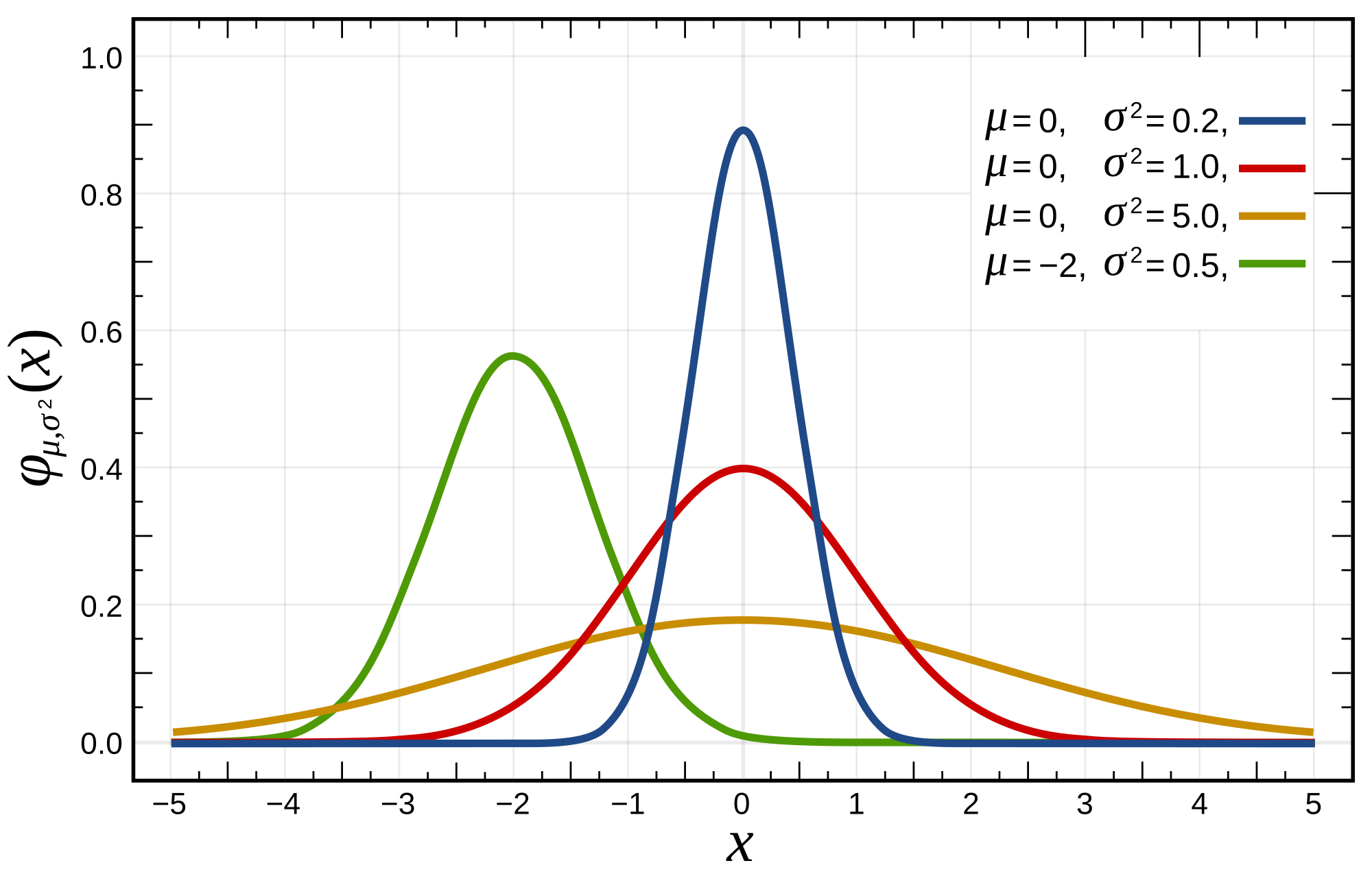
The parameter is the mean or expectation of the distribution (and also its median and mode), while the parameter is the variance. The standard deviation of the distribution is (sigma). A random variable with a Gaussian distribution is said to be normally distributed and is called a normal deviate.


Normal distributions are important in statistics and are often used in the natural and social sciences to represent real-valued random variables whose distributions are not known.[5][6] Their importance is partly due to the central limit theorem. It states that, under some conditions, the average of many samples (observations) of a random variable with finite mean and variance is itself a random variable—whose distribution converges to a normal distribution as the number of samples increases. Therefore, physical quantities that are expected to be the sum of many independent processes, such as measurement errors, often have distributions that are nearly normal.[7]
Moreover, Gaussian distributions have some unique properties that are valuable in analytic studies. For instance, any linear combination of a fixed collection of independent normal deviates is a normal deviate. Many results and methods, such as propagation of uncertainty and least squares[8] parameter fitting, can be derived analytically in explicit form when the relevant variables are normally distributed.
A normal distribution is sometimes informally called a bell curve.[9][10] However, many other distributions are bell-shaped (such as the Cauchy, Student's t, and logistic distributions). (For other names, see Naming.)
The univariate probability distribution is generalized for vectors in the multivariate normal distribution and for matrices in the matrix normal distribution.
Definitions
[edit]Standard normal distribution
[edit]The simplest case of a normal distribution is known as the standard normal distribution or unit normal distribution. This is a special case when and , and it is described by this probability density function (or density):[11] The variable has a mean of 0 and a variance and standard deviation of 1. The density has its peak at and inflection points at and .


Although the density above is most commonly known as the standard normal, a few authors have used that term to describe other versions of the normal distribution. Carl Friedrich Gauss, for example, once defined the standard normal as which has a variance of , and Stephen Stigler[12] once defined the standard normal as which has a simple functional form and a variance of


General normal distribution
[edit]Every normal distribution is a version of the standard normal distribution, whose domain has been stretched by a factor (the standard deviation) and then translated by (the mean value):

The probability density must be scaled by so that the integral is still 1.

If is a standard normal deviate, then will have a normal distribution with expected value and standard deviation . This is equivalent to saying that the standard normal distribution can be scaled/stretched by a factor of and shifted by to yield a different normal distribution, called . Conversely, if is a normal deviate with parameters and , then this distribution can be re-scaled and shifted via the formula to convert it to the standard normal distribution. This variate is also called the standardized form of .


Notation
[edit]The probability density of the standard Gaussian distribution (standard normal distribution, with zero mean and unit variance) is often denoted with the Greek letter (phi).[13] The alternative form of the Greek letter phi, , is also used quite often.


The normal distribution is often referred to as or .[14] Thus when a random variable is normally distributed with mean and standard deviation , one may write


Alternative parameterizations
[edit]Some authors advocate using the precision as the parameter defining the width of the distribution, instead of the standard deviation or the variance . The precision is normally defined as the reciprocal of the variance, .[15] The formula for the distribution then becomes


This choice is claimed to have advantages in numerical computations when is very close to zero, and simplifies formulas in some contexts, such as in the Bayesian inference of variables with multivariate normal distribution.
Alternatively, the reciprocal of the standard deviation might be defined as the precision, in which case the expression of the normal distribution becomes


According to Stigler, this formulation is advantageous because of a much simpler and easier-to-remember formula, and simple approximate formulas for the quantiles of the distribution.
Normal distributions form an exponential family with natural parameters and , and natural statistics x and x2. The dual expectation parameters for normal distribution are η1 = μ and η2 = μ2 + σ2.


Cumulative distribution function
[edit]The cumulative distribution function (CDF) of the standard normal distribution, usually denoted with the capital Greek letter , is the integral


Error function
[edit]The related error function gives the probability of a random variable, with normal distribution of mean 0 and variance 1/2 falling in the range . That is:

![{\displaystyle [-x,x]}](https://wikimedia.org/api/rest_v1/media/math/render/svg/e23c41ff0bd6f01a0e27054c2b85819fcd08b762)

These integrals cannot be expressed in terms of elementary functions, and are often said to be special functions. However, many numerical approximations are known; see below for more.
The two functions are closely related, namely
![{\displaystyle \Phi (x)={\frac {1}{2}}\left[1+\operatorname {erf} \left({\frac {x}{\sqrt {2}}}\right)\right]\,.}](https://wikimedia.org/api/rest_v1/media/math/render/svg/4dec6de19ebeaa734086622f167d87ac41e7b50d)
For a generic normal distribution with density , mean and variance , the cumulative distribution function is

![{\displaystyle F(x)=\Phi {\left({\frac {x-\mu }{\sigma }}\right)}={\frac {1}{2}}\left[1+\operatorname {erf} \left({\frac {x-\mu }{\sigma {\sqrt {2}}}}\right)\right]\,.}](https://wikimedia.org/api/rest_v1/media/math/render/svg/eabefd31d90af5221d89c397c7caef45a419b2bd)
The complement of the standard normal cumulative distribution function, , is often called the Q-function, especially in engineering texts.[16][17] It gives the probability that the value of a standard normal random variable will exceed : . Other definitions of the -function, all of which are simple transformations of , are also used occasionally.[18]


The graph of the standard normal cumulative distribution function has 2-fold rotational symmetry around the point (0,1/2); that is, . Its antiderivative (indefinite integral) can be expressed as follows:


The cumulative distribution function of the standard normal distribution can be expanded by integration by parts into a series:
![{\displaystyle \Phi (x)={\frac {1}{2}}+{\frac {1}{\sqrt {2\pi }}}\cdot e^{-x^{2}/2}\left[x+{\frac {x^{3}}{3}}+{\frac {x^{5}}{3\cdot 5}}+\cdots +{\frac {x^{2n+1}}{(2n+1)!!}}+\cdots \right]\,.}](https://wikimedia.org/api/rest_v1/media/math/render/svg/ad8275ec6180f68c2dae03c9e70716b75ff4f3aa)
where denotes the double factorial.

An asymptotic expansion of the cumulative distribution function for large x can also be derived using integration by parts. For more, see Error function § Asymptotic expansion.[19]
A quick approximation to the standard normal distribution's cumulative distribution function can be found by using a Taylor series approximation:

Recursive computation with Taylor series expansion
[edit]The recursive nature of the family of derivatives may be used to easily construct a rapidly converging Taylor series expansion using recursive entries about any point of known value of the distribution,:


where:

Using the Taylor series and Newton's method for the inverse function
[edit]An application for the above Taylor series expansion is to use Newton's method to reverse the computation. That is, if we have a value for the cumulative distribution function, , but do not know the x needed to obtain the , we can use Newton's method to find x, and use the Taylor series expansion above to minimize the number of computations. Newton's method is ideal to solve this problem because the first derivative of , which is an integral of the normal standard distribution, is the normal standard distribution, and is readily available to use in the Newton's method solution.

To solve, select a known approximate solution, , to the desired . may be a value from a distribution table, or an intelligent estimate followed by a computation of using any desired means to compute. Use this value of and the Taylor series expansion above to minimize computations.


Repeat the following process until the difference between the computed and the desired , which we will call , is below a chosen acceptably small error, such as 10−5, 10−15, etc.:


where
- is the from a Taylor series solution using and


When the repeated computations converge to an error below the chosen acceptably small value, x will be the value needed to obtain a of the desired value, .

Standard deviation and coverage
[edit]
About 68% of values drawn from a normal distribution are within one standard deviation σ from the mean; about 95% of the values lie within two standard deviations; and about 99.7% are within three standard deviations.[9] This fact is known as the 68–95–99.7 (empirical) rule, or the 3-sigma rule.
More precisely, the probability that a normal deviate lies in the range between and is given by To 12 significant digits, the values for are:


| | OEIS | |||||
|---|---|---|---|---|---|---|
| 1 | 0.682689492137 | 0.317310507863 |
|
OEIS: A178647 | ||
| 2 | 0.954499736104 | 0.045500263896 |
|
OEIS: A110894 | ||
| 3 | 0.997300203937 | 0.002699796063 |
|
OEIS: A270712 | ||
| 4 | 0.999936657516 | 0.000063342484 |
| |||
| 5 | 0.999999426697 | 0.000000573303 |
| |||
| 6 | 0.999999998027 | 0.000000001973 |
|


For large , one can use the approximation .

Quantile function
[edit]The quantile function of a distribution is the inverse of the cumulative distribution function. The quantile function of the standard normal distribution is called the probit function, and can be expressed in terms of the inverse error function: For a normal random variable with mean and variance , the quantile function is The quantile of the standard normal distribution is commonly denoted as . These values are used in hypothesis testing, construction of confidence intervals and Q–Q plots. A normal random variable will exceed with probability , and will lie outside the interval with probability . In particular, the quantile is 1.96; therefore a normal random variable will lie outside the interval in only 5% of cases.


The following table gives the quantile such that will lie in the range with a specified probability . These values are useful to determine tolerance interval for sample averages and other statistical estimators with normal (or asymptotically normal) distributions.[20] The following table shows , not as defined above.


| | | |||
|---|---|---|---|---|
| 0.80 | 1.281551565545 | 0.999 | 3.290526731492 | |
| 0.90 | 1.644853626951 | 0.9999 | 3.890591886413 | |
| 0.95 | 1.959963984540 | 0.99999 | 4.417173413469 | |
| 0.98 | 2.326347874041 | 0.999999 | 4.891638475699 | |
| 0.99 | 2.575829303549 | 0.9999999 | 5.326723886384 | |
| 0.995 | 2.807033768344 | 0.99999999 | 5.730728868236 | |
| 0.998 | 3.090232306168 | 0.999999999 | 6.109410204869 |
For small , the quantile function has the useful asymptotic expansion [citation needed]

Properties
[edit]The normal distribution is the only distribution whose cumulants beyond the first two (i.e., other than the mean and variance) are zero. It is also the continuous distribution with the maximum entropy for a specified mean and variance.[21][22] Geary has shown, assuming that the mean and variance are finite, that the normal distribution is the only distribution where the mean and variance calculated from a set of independent draws are independent of each other.[23][24]
The normal distribution is a subclass of the elliptical distributions. The normal distribution is symmetric about its mean, and is non-zero over the entire real line. As such it may not be a suitable model for variables that are inherently positive or strongly skewed, such as the weight of a person or the price of a share. Such variables may be better described by other distributions, such as the log-normal distribution or the Pareto distribution.
The value of the normal density is practically zero when the value lies more than a few standard deviations away from the mean (e.g., a spread of three standard deviations covers all but 0.27% of the total distribution). Therefore, it may not be an appropriate model when one expects a significant fraction of outliers—values that lie many standard deviations away from the mean—and least squares and other statistical inference methods that are optimal for normally distributed variables often become highly unreliable when applied to such data. In those cases, a more heavy-tailed distribution should be assumed and the appropriate robust statistical inference methods applied.
The Gaussian distribution belongs to the family of stable distributions which are the attractors of sums of independent, identically distributed distributions whether or not the mean or variance is finite. Except for the Gaussian which is a limiting case, all stable distributions have heavy tails and infinite variance. It is one of the few distributions that are stable and that have probability density functions that can be expressed analytically, the others being the Cauchy distribution and the Lévy distribution.
Symmetries and derivatives
[edit]The normal distribution with density (mean and variance ) has the following properties:


- It is symmetric around the point which is at the same time the mode, the median and the mean of the distribution.[25]
- It is unimodal: its first derivative is positive for negative for and zero only at
- The area bounded by the curve and the -axis is unity (i.e. equal to one).
- Its first derivative is
- Its second derivative is
- Its density has two inflection points (where the second derivative of is zero and changes sign), located one standard deviation away from the mean, namely at and [25]
- Its density is log-concave.[25]
- Its density is infinitely differentiable, indeed supersmooth of order 2.[26]


Furthermore, the density of the standard normal distribution (i.e. and ) also has the following properties:

- Its first derivative is
- Its second derivative is
- More generally, its nth derivative is where is the nth (probabilist) Hermite polynomial.[27]
- The probability that a normally distributed variable with known and is in a particular set, can be calculated by using the fact that the fraction has a standard normal distribution.


Moments
[edit]The plain and absolute moments of a variable are the expected values of and , respectively. If the expected value of is zero, these parameters are called central moments; otherwise, these parameters are called non-central moments. Usually we are interested only in moments with integer order .


If has a normal distribution, the non-central moments exist and are finite for any whose real part is greater than −1. For any non-negative integer , the plain central moments are:[28] Here denotes the double factorial, that is, the product of all numbers from to 1 that have the same parity as
![{\displaystyle \operatorname {E} \left[(X-\mu )^{p}\right]={\begin{cases}0&{\text{if }}p{\text{ is odd,}}\\\sigma ^{p}(p-1)!!&{\text{if }}p{\text{ is even.}}\end{cases}}}](https://wikimedia.org/api/rest_v1/media/math/render/svg/f1d2c92b62ac2bbe07a8e475faac29c8cc5f7755)


The central absolute moments coincide with plain moments for all even orders, but are nonzero for odd orders. For any non-negative integer

The last formula is valid also for any non-integer When the mean the plain and absolute moments can be expressed in terms of confluent hypergeometric functions and [29]
![{\displaystyle {\begin{aligned}\operatorname {E} \left[|X-\mu |^{p}\right]&=\sigma ^{p}(p-1)!!\cdot {\begin{cases}{\sqrt {\frac {2}{\pi }}}&{\text{if }}p{\text{ is odd}}\\1&{\text{if }}p{\text{ is even}}\end{cases}}\\&=\sigma ^{p}\cdot {\frac {2^{p/2}\Gamma \left({\frac {p+1}{2}}\right)}{\sqrt {\pi }}}.\end{aligned}}}](https://wikimedia.org/api/rest_v1/media/math/render/svg/3b196371c491676efa7ea7770ef56773db7652cd)


![{\displaystyle {\begin{aligned}\operatorname {E} \left[X^{p}\right]&=\sigma ^{p}\cdot {\left(-i{\sqrt {2}}\right)}^{p}\,U{\left(-{\frac {p}{2}},{\frac {1}{2}},-{\frac {\mu ^{2}}{2\sigma ^{2}}}\right)},\\\operatorname {E} \left[|X|^{p}\right]&=\sigma ^{p}\cdot 2^{p/2}{\frac {\Gamma {\left({\frac {1+p}{2}}\right)}}{\sqrt {\pi }}}\,{}_{1}F_{1}{\left(-{\frac {p}{2}},{\frac {1}{2}},-{\frac {\mu ^{2}}{2\sigma ^{2}}}\right)}.\end{aligned}}}](https://wikimedia.org/api/rest_v1/media/math/render/svg/7c1a76b43032d0b01ff1935cced240253263ec62)
These expressions remain valid even if is not an integer. See also generalized Hermite polynomials.
| Order | Non-central moment, | Central moment, |
|---|---|---|
| 0 | | |
| 1 | | |
| 2 | ||
| 3 | | |
| 4 | ||
| 5 | | |
| 6 | ||
| 7 | | |
| 8 |
![{\displaystyle \operatorname {E} \left[X^{p}\right]}](https://wikimedia.org/api/rest_v1/media/math/render/svg/53264b5ab94e93f2e7de05de69012af27df4c4f4)
![{\displaystyle \operatorname {E} \left[(X-\mu )^{p}\right]}](https://wikimedia.org/api/rest_v1/media/math/render/svg/598b838fed4500017abb513a203a89999c74ce22)


The expectation of conditioned on the event that lies in an interval is given by where and respectively are the density and the cumulative distribution function of . For this is known as the inverse Mills ratio. Note that above, density of is used instead of standard normal density as in inverse Mills ratio, so here we have instead of .
![{\textstyle [a,b]}](https://wikimedia.org/api/rest_v1/media/math/render/svg/2c780cbaafb5b1d4a6912aa65d2b0b1982097108)
![{\displaystyle \operatorname {E} \left[X\mid a<X<b\right]=\mu -\sigma ^{2}{\frac {f(b)-f(a)}{F(b)-F(a)}}\,,}](https://wikimedia.org/api/rest_v1/media/math/render/svg/ad97cc40960e6d1d4e65f51596c9cd0c9accfdc0)


Fourier transform and characteristic function
[edit]The Fourier transform of a normal density with mean and variance is[30]

where is the imaginary unit. If the mean , the first factor is 1, and the Fourier transform is, apart from a constant factor, a normal density on the frequency domain, with mean 0 and variance . In particular, the standard normal distribution is an eigenfunction of the Fourier transform.

In probability theory, the Fourier transform of the probability distribution of a real-valued random variable is closely connected to the characteristic function of that variable, which is defined as the expected value of , as a function of the real variable (the frequency parameter of the Fourier transform). This definition can be analytically extended to a complex-value variable .[31] The relation between both is:


The real and imaginary parts of give:
![{\displaystyle {\hat {f}}(t)=\operatorname {E} [e^{-itx}]=e^{-i\mu t}e^{-{\frac {1}{2}}\sigma ^{2}t^{2}}}](https://wikimedia.org/api/rest_v1/media/math/render/svg/952332f7eee9e208a58adcb0fc9579bdaa143cce)
- and
- .
![{\displaystyle \operatorname {E} [\cos(tx)]=\cos(\mu t)e^{-{\frac {1}{2}}\sigma ^{2}t^{2}}}](https://wikimedia.org/api/rest_v1/media/math/render/svg/5395d7de6a6755a20b760ae1a32fffc4321f63be)
![{\displaystyle \operatorname {E} [\sin(tx)]=\sin(\mu t)e^{-{\frac {1}{2}}\sigma ^{2}t^{2}}}](https://wikimedia.org/api/rest_v1/media/math/render/svg/b0507996e8e86f17b96c2ebe2642669246b687c4)
Similarly,
- and
- .
![{\displaystyle \operatorname {E} [\cosh(tx)]=\cosh(\mu t)e^{{\frac {1}{2}}\sigma ^{2}t^{2}}}](https://wikimedia.org/api/rest_v1/media/math/render/svg/ab17a3e9ea7d35d5f8f142bdb6057ea1cf8ff224)
![{\displaystyle \operatorname {E} [\sinh(tx)]=\sinh(\mu t)e^{{\frac {1}{2}}\sigma ^{2}t^{2}}}](https://wikimedia.org/api/rest_v1/media/math/render/svg/89b7445bb38d3dceb7bb7633a990eea293e4b6a1)
These formulas evaluated at give the expected value of these basic trigonometric and hyperbolic functions over a Gaussian random variable , which also could be seen as consequences of the Isserlis's theorem.


Moment- and cumulant-generating functions
[edit]The moment generating function of a real random variable is the expected value of , as a function of the real parameter . For a normal distribution with density , mean and variance , the moment generating function exists and is equal to

For any , the coefficient of in the moment generating function (expressed as an exponential power series in ) is the normal distribution's expected value .
![{\displaystyle M(t)=\operatorname {E} \left[e^{tX}\right]={\hat {f}}(it)=e^{\mu t}e^{\sigma ^{2}t^{2}/2}\,.}](https://wikimedia.org/api/rest_v1/media/math/render/svg/3b5930b107fb4328bc04d077d65ce3d2bf1510de)


![{\displaystyle \operatorname {E} [X^{k}]}](https://wikimedia.org/api/rest_v1/media/math/render/svg/9893a5b728d8111751abbcf6bd653d214b462cdc)
The cumulant generating function is the logarithm of the moment generating function, namely

The coefficients of this exponential power series define the cumulants, but because this is a quadratic polynomial in , only the first two cumulants are nonzero, namely the mean and the variance .
Some authors prefer to instead work with the characteristic function E[eitX] = eiμt − σ2t2/2 and ln E[eitX] = iμt − 1/2σ2t2.
Stein operator and class
[edit]Within Stein's method the Stein operator and class of a random variable are and the class of all absolutely continuous functions such that .


![{\displaystyle \operatorname {E} [\vert f'(X)\vert ]<\infty }](https://wikimedia.org/api/rest_v1/media/math/render/svg/c172f331ab4cca02c7e06a7322b7832f082e717b)
Zero-variance limit
[edit]In the limit when approaches zero, the probability density approaches zero everywhere except at , where it approaches , while its integral remains equal to 1. An extension of the normal distribution to the case with zero variance can be defined using the Dirac delta measure , although the resulting random variables are not absolutely continuous and thus do not have probability density functions. The cumulative distribution function of such a random variable is then the Heaviside step function translated by the mean , namely


Maximum entropy
[edit]Of all probability distributions over the reals with a specified finite mean and finite variance , the normal distribution is the one with maximum entropy.[21] To see this, let be a continuous random variable with probability density . The entropy of is defined as[32][33][34]


where is understood to be zero whenever . This functional can be maximized, subject to the constraints that the distribution is properly normalized and has a specified mean and variance, by using variational calculus. A function with three Lagrange multipliers is defined:


At maximum entropy, a small variation about will produce a variation about which is equal to 0:


Since this must hold for any small , the factor multiplying must be zero, and solving for yields:


The Lagrange constraints that is properly normalized and has the specified mean and variance are satisfied if and only if , , and are chosen so that The entropy of a normal distribution is equal to which is independent of the mean .


Other properties
[edit]- If the characteristic function of some random variable is of the form in a neighborhood of zero, where is a polynomial, then the Marcinkiewicz theorem (named after Józef Marcinkiewicz) asserts that can be at most a quadratic polynomial, and therefore is a normal random variable.[35] The consequence of this result is that the normal distribution is the only distribution with a finite number (two) of non-zero cumulants.
- If and are jointly normal and uncorrelated, then they are independent. The requirement that and should be jointly normal is essential; without it the property does not hold.[36][37][proof] For non-normal random variables uncorrelatedness does not imply independence.
- The Kullback–Leibler divergence of one normal distribution from another is given by:[38] The Hellinger distance between the same distributions is equal to
- The Fisher information matrix for a normal distribution w.r.t. and is diagonal and takes the form
- The conjugate prior of the mean of a normal distribution is another normal distribution.[39] Specifically, if are iid and the prior is , then the posterior distribution for the estimator of will be
- The family of normal distributions not only forms an exponential family (EF), but in fact forms a natural exponential family (NEF) with quadratic variance function (NEF-QVF). Many properties of normal distributions generalize to properties of NEF-QVF distributions, NEF distributions, or EF distributions generally. NEF-QVF distributions comprises 6 families, including Poisson, Gamma, binomial, and negative binomial distributions, while many of the common families studied in probability and statistics are NEF or EF.
- In information geometry, the family of normal distributions forms a statistical manifold with constant curvature . The same family is flat with respect to the (±1)-connections and .[40]
- If are distributed according to , then . Note that there is no assumption of independence.[41]


![{\textstyle E[\max _{i}X_{i}]\leq \sigma {\sqrt {2\ln n}}}](https://wikimedia.org/api/rest_v1/media/math/render/svg/0dfb87c9b047ccf23ace2139d97810dff1ed6670)
Related distributions
[edit]Central limit theorem
[edit]

The central limit theorem states that under certain (fairly common) conditions, the sum of many random variables will have an approximately normal distribution. More specifically, where are independent and identically distributed random variables with the same arbitrary distribution, zero mean, and variance and is their mean scaled by Then, as increases, the probability distribution of will tend to the normal distribution with zero mean and variance .


The theorem can be extended to variables that are not independent and/or not identically distributed if certain constraints are placed on the degree of dependence and the moments of the distributions.

Many test statistics, scores, and estimators encountered in practice contain sums of certain random variables in them, and even more estimators can be represented as sums of random variables through the use of influence functions. The central limit theorem implies that those statistical parameters will have asymptotically normal distributions.
The central limit theorem also implies that certain distributions can be approximated by the normal distribution, for example:
- The binomial distribution is approximately normal with mean and variance for large and for not too close to 0 or 1.
- The Poisson distribution with parameter is approximately normal with mean and variance , for large values of .[42]
- The chi-squared distribution is approximately normal with mean and variance , for large .
- The Student's t-distribution is approximately normal with mean 0 and variance 1 when is large.


Whether these approximations are sufficiently accurate depends on the purpose for which they are needed, and the rate of convergence to the normal distribution. It is typically the case that such approximations are less accurate in the tails of the distribution.
A general upper bound for the approximation error in the central limit theorem is given by the Berry–Esseen theorem, improvements of the approximation are given by the Edgeworth expansions.
This theorem can also be used to justify modeling the sum of many uniform noise sources as Gaussian noise. See AWGN.
Operations and functions of normal variables
[edit]
x = 10, σ2
y = 20, and ρxy = 0.495. d: Probability density of a function |x1| + ... + |x4| of four iid standard normal variables. These are computed by the numerical method of ray-tracing.[43]
The probability density, cumulative distribution, and inverse cumulative distribution of any function of one or more independent or correlated normal variables can be computed with the numerical method of ray-tracing[43] (Matlab code). In the following sections we look at some special cases.
Operations on a single normal variable
[edit]If is distributed normally with mean and variance , then
- , for any real numbers and , is also normally distributed, with mean and variance . That is, the family of normal distributions is closed under linear transformations.
- The exponential of is distributed log-normally: .
- The standard sigmoid of is logit-normally distributed: .
- The absolute value of has folded normal distribution: . If this is known as the half-normal distribution.
- The absolute value of normalized residuals, , has chi distribution with one degree of freedom: .
- The square of has the noncentral chi-squared distribution with one degree of freedom: . If , the distribution is called simply chi-squared.
- The log-likelihood of a normal variable is simply the log of its probability density function: Since this is a scaled and shifted square of a standard normal variable, it is distributed as a scaled and shifted chi-squared variable.
- The distribution of the variable restricted to an interval is called the truncated normal distribution.
- has a Lévy distribution with location 0 and scale .


Operations on two independent normal variables
[edit]- If and are two independent normal random variables, with means , and variances , , then their sum will also be normally distributed,[proof] with mean and variance .
- In particular, if and are independent normal deviates with zero mean and variance , then and are also independent and normally distributed, with zero mean and variance . This is a special case of the polarization identity.[44]
- If , are two independent normal deviates with mean and variance , and , are arbitrary real numbers, then the variable is also normally distributed with mean and variance . It follows that the normal distribution is stable (with exponent ).
- If , are normal distributions, then their normalized geometric mean is a normal distribution with and .


Operations on two independent standard normal variables
[edit]If and are two independent standard normal random variables with mean 0 and variance 1, then
- Their sum and difference is distributed normally with mean zero and variance two: .
- Their product follows the product distribution[45] with density function where is the modified Bessel function of the second kind. This distribution is symmetric around zero, unbounded at , and has the characteristic function .
- Their ratio follows the standard Cauchy distribution: .
- Their Euclidean norm has the Rayleigh distribution.


Operations on multiple independent normal variables
[edit]- Any linear combination of independent normal deviates is a normal deviate.
- If are independent standard normal random variables, then the sum of their squares has the chi-squared distribution with degrees of freedom
- If are independent normally distributed random variables with means and variances , then their sample mean is independent from the sample standard deviation,[46] which can be demonstrated using Basu's theorem or Cochran's theorem.[47] The ratio of these two quantities will have the Student's t-distribution with degrees of freedom:
- If , are independent standard normal random variables, then the ratio of their normalized sums of squares will have the F-distribution with (n, m) degrees of freedom:[48]


![{\displaystyle t={\frac {{\overline {X}}-\mu }{S/{\sqrt {n}}}}={\frac {{\frac {1}{n}}(X_{1}+\cdots +X_{n})-\mu }{\sqrt {{\frac {1}{n(n-1)}}\left[(X_{1}-{\overline {X}})^{2}+\cdots +(X_{n}-{\overline {X}})^{2}\right]}}}\sim t_{n-1}.}](https://wikimedia.org/api/rest_v1/media/math/render/svg/36ff0d3c79a0504e8f259ef99192b825357914d7)


Operations on multiple correlated normal variables
[edit]- A quadratic form of a normal vector, i.e. a quadratic function of multiple independent or correlated normal variables, is a generalized chi-square variable.

Operations on the density function
[edit]The split normal distribution is most directly defined in terms of joining scaled sections of the density functions of different normal distributions and rescaling the density to integrate to one. The truncated normal distribution results from rescaling a section of a single density function.
Infinite divisibility and Cramér's theorem
[edit]For any positive integer n, any normal distribution with mean and variance is the distribution of the sum of n independent normal deviates, each with mean and variance . This property is called infinite divisibility.[49]


Conversely, if and are independent random variables and their sum has a normal distribution, then both and must be normal deviates.[50]
This result is known as Cramér's decomposition theorem, and is equivalent to saying that the convolution of two distributions is normal if and only if both are normal. Cramér's theorem implies that a linear combination of independent non-Gaussian variables will never have an exactly normal distribution, although it may approach it arbitrarily closely.[35]
The Kac–Bernstein theorem
[edit]The Kac–Bernstein theorem states that if and are independent and and are also independent, then both X and Y must necessarily have normal distributions.[51][52]

More generally, if are independent random variables, then two distinct linear combinations and will be independent if and only if all are normal and , where denotes the variance of .[51]


Extensions
[edit]The notion of normal distribution, being one of the most important distributions in probability theory, has been extended far beyond the standard framework of the univariate (that is one-dimensional) case (Case 1). All these extensions are also called normal or Gaussian laws, so a certain ambiguity in names exists.
- The multivariate normal distribution describes the Gaussian law in the k-dimensional Euclidean space. A vector X ∈ Rk is multivariate-normally distributed if any linear combination of its components Σk
j=1aj Xj has a (univariate) normal distribution. The variance of X is a k × k symmetric positive-definite matrix V. The multivariate normal distribution is a special case of the elliptical distributions. As such, its iso-density loci in the k = 2 case are ellipses and in the case of arbitrary k are ellipsoids. - Rectified Gaussian distribution a rectified version of normal distribution with all the negative elements reset to 0.
- Complex normal distribution deals with the complex normal vectors. A complex vector X ∈ Ck is said to be normal if both its real and imaginary components jointly possess a 2k-dimensional multivariate normal distribution. The variance-covariance structure of X is described by two matrices: the variance matrix Γ, and the relation matrix C.
- Matrix normal distribution describes the case of normally distributed matrices.
- Gaussian processes are the normally distributed stochastic processes. These can be viewed as elements of some infinite-dimensional Hilbert space H, and thus are the analogues of multivariate normal vectors for the case k = ∞. A random element h ∈ H is said to be normal if for any constant a ∈ H the scalar product (a, h) has a (univariate) normal distribution. The variance structure of such Gaussian random element can be described in terms of the linear covariance operator K: H → H. Several Gaussian processes became popular enough to have their own names:
- Gaussian q-distribution is an abstract mathematical construction that represents a q-analogue of the normal distribution.
- the q-Gaussian is an analogue of the Gaussian distribution, in the sense that it maximises the Tsallis entropy, and is one type of Tsallis distribution. This distribution is different from the Gaussian q-distribution above.
- The Kaniadakis κ-Gaussian distribution is a generalization of the Gaussian distribution which arises from the Kaniadakis statistics, being one of the Kaniadakis distributions.
A random variable X has a two-piece normal distribution if it has a distribution

where μ is the mean and σ2
1 and σ2
2 are the variances of the distribution to the left and right of the mean respectively.
The mean E(X), variance V(X), and third central moment T(X) of this distribution have been determined[53]
![{\displaystyle {\begin{aligned}\operatorname {E} (X)&=\mu +{\sqrt {\frac {2}{\pi }}}(\sigma _{2}-\sigma _{1}),\\\operatorname {V} (X)&=\left(1-{\frac {2}{\pi }}\right)(\sigma _{2}-\sigma _{1})^{2}+\sigma _{1}\sigma _{2},\\\operatorname {T} (X)&={\sqrt {\frac {2}{\pi }}}(\sigma _{2}-\sigma _{1})\left[\left({\frac {4}{\pi }}-1\right)(\sigma _{2}-\sigma _{1})^{2}+\sigma _{1}\sigma _{2}\right].\end{aligned}}}](https://wikimedia.org/api/rest_v1/media/math/render/svg/97f32cc8147bff0b5cdc02123a520a1119854060)
One of the main practical uses of the Gaussian law is to model the empirical distributions of many different random variables encountered in practice. In such case a possible extension would be a richer family of distributions, having more than two parameters and therefore being able to fit the empirical distribution more accurately. The examples of such extensions are:
- Pearson distribution — a four-parameter family of probability distributions that extend the normal law to include different skewness and kurtosis values.
- The generalized normal distribution, also known as the exponential power distribution, allows for distribution tails with thicker or thinner asymptotic behaviors.
Statistical inference
[edit]Estimation of parameters
[edit]It is often the case that we do not know the parameters of the normal distribution, but instead want to estimate them. That is, having a sample from a normal population we would like to learn the approximate values of parameters and . The standard approach to this problem is the maximum likelihood method, which requires maximization of the log-likelihood function: Taking derivatives with respect to and and solving the resulting system of first order conditions yields the maximum likelihood estimates:


Then is as follows:

![{\displaystyle \ln {\mathcal {L}}({\hat {\mu }},{\hat {\sigma }}^{2})=(-n/2)[\ln(2\pi {\hat {\sigma }}^{2})+1]}](https://wikimedia.org/api/rest_v1/media/math/render/svg/561353e6bc80d226fddd9510be61d21bc67b3aee)
Sample mean
[edit]Estimator is called the sample mean, since it is the arithmetic mean of all observations. The statistic is complete and sufficient for , and therefore by the Lehmann–Scheffé theorem, is the uniformly minimum variance unbiased (UMVU) estimator.[54] In finite samples it is distributed normally: The variance of this estimator is equal to the μμ-element of the inverse Fisher information matrix . This implies that the estimator is finite-sample efficient. Of practical importance is the fact that the standard error of is proportional to , that is, if one wishes to decrease the standard error by a factor of 10, one must increase the number of points in the sample by a factor of 100. This fact is widely used in determining sample sizes for opinion polls and the number of trials in Monte Carlo simulations.


From the standpoint of the asymptotic theory, is consistent, that is, it converges in probability to as . The estimator is also asymptotically normal, which is a simple corollary of the fact that it is normal in finite samples:


Sample variance
[edit]The estimator is called the sample variance, since it is the variance of the sample (). In practice, another estimator is often used instead of the . This other estimator is denoted , and is also called the sample variance, which represents a certain ambiguity in terminology; its square root is called the sample standard deviation. The estimator differs from by having (n − 1) instead of n in the denominator (the so-called Bessel's correction): The difference between and becomes negligibly small for large n's. In finite samples however, the motivation behind the use of is that it is an unbiased estimator of the underlying parameter , whereas is biased. Also, by the Lehmann–Scheffé theorem the estimator is uniformly minimum variance unbiased (UMVU),[54] which makes it the "best" estimator among all unbiased ones. However it can be shown that the biased estimator is better than the in terms of the mean squared error (MSE) criterion. In finite samples both and have scaled chi-squared distribution with (n − 1) degrees of freedom: The first of these expressions shows that the variance of is equal to , which is slightly greater than the σσ-element of the inverse Fisher information matrix , which is . Thus, is not an efficient estimator for , and moreover, since is UMVU, we can conclude that the finite-sample efficient estimator for does not exist.


Applying the asymptotic theory, both estimators and are consistent, that is they converge in probability to as the sample size . The two estimators are also both asymptotically normal: In particular, both estimators are asymptotically efficient for .

Confidence intervals
[edit]By Cochran's theorem, for normal distributions the sample mean and the sample variance s2 are independent, which means there can be no gain in considering their joint distribution. There is also a converse theorem: if in a sample the sample mean and sample variance are independent, then the sample must have come from the normal distribution. The independence between and s can be employed to construct the so-called t-statistic:
This quantity t has the Student's t-distribution with (n − 1) degrees of freedom, and it is an ancillary statistic (independent of the value of the parameters). Inverting the distribution of this t-statistics will allow us to construct the confidence interval for μ;[55] similarly, inverting the χ2 distribution of the statistic s2 will give us the confidence interval for σ2:[56]
where tk,p and χ 2
k,p are the pth quantiles of the t- and χ2-distributions respectively. These confidence intervals are of the confidence level 1 − α, meaning that the true values μ and σ2 fall outside of these intervals with probability (or significance level) α. In practice people usually take α = 5%, resulting in the 95% confidence intervals. The confidence interval for σ can be found by taking the square root of the interval bounds for σ2.

![{\displaystyle \mu \in \left[{\hat {\mu }}-t_{n-1,1-\alpha /2}{\frac {s}{\sqrt {n}}},\,{\hat {\mu }}+t_{n-1,1-\alpha /2}{\frac {s}{\sqrt {n}}}\right]}](https://wikimedia.org/api/rest_v1/media/math/render/svg/86ad00c4aac2907f6358d3ab3a5e413a58158be4)
![{\displaystyle \sigma ^{2}\in \left[{\frac {n-1}{\chi _{n-1,1-\alpha /2}^{2}}}s^{2},\,{\frac {n-1}{\chi _{n-1,\alpha /2}^{2}}}s^{2}\right]}](https://wikimedia.org/api/rest_v1/media/math/render/svg/87c0c6ae7bd48ba8377279fed58df479f0de900c)
Approximate formulas can be derived from the asymptotic distributions of and s2: The approximate formulas become valid for large values of n, and are more convenient for the manual calculation since the standard normal quantiles zα/2 do not depend on n. In particular, the most popular value of α = 5%, results in |z0.025| = 1.96.
![{\displaystyle \mu \in \left[{\hat {\mu }}-{\frac {|z_{\alpha /2}|}{\sqrt {n}}}s,\,{\hat {\mu }}+{\frac {|z_{\alpha /2}|}{\sqrt {n}}}s\right]}](https://wikimedia.org/api/rest_v1/media/math/render/svg/6ed5adb135a9cd03de1aa21d774e66be1adb4ea8)
![{\displaystyle \sigma ^{2}\in \left[s^{2}-{\sqrt {2}}{\frac {|z_{\alpha /2}|}{\sqrt {n}}}s^{2},\,s^{2}+{\sqrt {2}}{\frac {|z_{\alpha /2}|}{\sqrt {n}}}s^{2}\right]}](https://wikimedia.org/api/rest_v1/media/math/render/svg/56646fb560578a0414ad2f045c14031c4015b9a2)
Normality tests
[edit]Normality tests assess the likelihood that the given data set {x1, ..., xn} comes from a normal distribution. Typically the null hypothesis H0 is that the observations are distributed normally with unspecified mean μ and variance σ2, versus the alternative Ha that the distribution is arbitrary. Many tests (over 40) have been devised for this problem. The more prominent of them are outlined below:
Diagnostic plots are more intuitively appealing but subjective at the same time, as they rely on informal human judgement to accept or reject the null hypothesis.
- Q–Q plot, also known as normal probability plot or rankit plot—is a plot of the sorted values from the data set against the expected values of the corresponding quantiles from the standard normal distribution. That is, it is a plot of point of the form (Φ−1(pk), x(k)), where plotting points pk are equal to pk = (k − α)/(n + 1 − 2α) and α is an adjustment constant, which can be anything between 0 and 1. If the null hypothesis is true, the plotted points should approximately lie on a straight line.
- P–P plot – similar to the Q–Q plot, but used much less frequently. This method consists of plotting the points (Φ(z(k)), pk), where . For normally distributed data this plot should lie on a 45° line between (0, 0) and (1, 1).

Goodness-of-fit tests:
Moment-based tests:
- D'Agostino's K-squared test
- Jarque–Bera test
- Shapiro–Wilk test: This is based on the fact that the line in the Q–Q plot has the slope of σ. The test compares the least squares estimate of that slope with the value of the sample variance, and rejects the null hypothesis if these two quantities differ significantly.
Tests based on the empirical distribution function:
- Anderson–Darling test
- Lilliefors test (an adaptation of the Kolmogorov–Smirnov test)
Bayesian analysis of the normal distribution
[edit]Bayesian analysis of normally distributed data is complicated by the many different possibilities that may be considered:
- Either the mean, or the variance, or neither, may be considered a fixed quantity.
- When the variance is unknown, analysis may be done directly in terms of the variance, or in terms of the precision, the reciprocal of the variance. The reason for expressing the formulas in terms of precision is that the analysis of most cases is simplified.
- Both univariate and multivariate cases need to be considered.
- Either conjugate or improper prior distributions may be placed on the unknown variables.
- An additional set of cases occurs in Bayesian linear regression, where in the basic model the data is assumed to be normally distributed, and normal priors are placed on the regression coefficients. The resulting analysis is similar to the basic cases of independent identically distributed data.
The formulas for the non-linear-regression cases are summarized in the conjugate prior article.
Sum of two quadratics
[edit]Scalar form
[edit]The following auxiliary formula is useful for simplifying the posterior update equations, which otherwise become fairly tedious.

This equation rewrites the sum of two quadratics in x by expanding the squares, grouping the terms in x, and completing the square. Note the following about the complex constant factors attached to some of the terms:
- The factor has the form of a weighted average of y and z.
- This shows that this factor can be thought of as resulting from a situation where the reciprocals of quantities a and b add directly, so to combine a and b themselves, it is necessary to reciprocate, add, and reciprocate the result again to get back into the original units. This is exactly the sort of operation performed by the harmonic mean, so it is not surprising that is one-half the harmonic mean of a and b.


Vector form
[edit]A similar formula can be written for the sum of two vector quadratics: If x, y, z are vectors of length k, and A and B are symmetric, invertible matrices of size , then


where

The form x′ A x is called a quadratic form and is a scalar: In other words, it sums up all possible combinations of products of pairs of elements from x, with a separate coefficient for each. In addition, since , only the sum matters for any off-diagonal elements of A, and there is no loss of generality in assuming that A is symmetric. Furthermore, if A is symmetric, then the form


Sum of differences from the mean
[edit]Another useful formula is as follows: where


With known variance
[edit]For a set of i.i.d. normally distributed data points X of size n where each individual point x follows with known variance σ2, the conjugate prior distribution is also normally distributed.

This can be shown more easily by rewriting the variance as the precision, i.e. using τ = 1/σ2. Then if and we proceed as follows.


First, the likelihood function is (using the formula above for the sum of differences from the mean):
![{\displaystyle {\begin{aligned}p(\mathbf {X} \mid \mu ,\tau )&=\prod _{i=1}^{n}{\sqrt {\frac {\tau }{2\pi }}}\exp \left(-{\frac {1}{2}}\tau (x_{i}-\mu )^{2}\right)\\&=\left({\frac {\tau }{2\pi }}\right)^{n/2}\exp \left(-{\frac {1}{2}}\tau \sum _{i=1}^{n}(x_{i}-\mu )^{2}\right)\\&=\left({\frac {\tau }{2\pi }}\right)^{n/2}\exp \left[-{\frac {1}{2}}\tau \left(\sum _{i=1}^{n}(x_{i}-{\bar {x}})^{2}+n({\bar {x}}-\mu )^{2}\right)\right].\end{aligned}}}](https://wikimedia.org/api/rest_v1/media/math/render/svg/c2bcd1c34520a24e29b758a0f7427e79e9d8a414)
Then, we proceed as follows:
![{\displaystyle {\begin{aligned}p(\mu \mid \mathbf {X} )&\propto p(\mathbf {X} \mid \mu )p(\mu )\\&=\left({\frac {\tau }{2\pi }}\right)^{n/2}\exp \left[-{\frac {1}{2}}\tau \left(\sum _{i=1}^{n}(x_{i}-{\bar {x}})^{2}+n({\bar {x}}-\mu )^{2}\right)\right]{\sqrt {\frac {\tau _{0}}{2\pi }}}\exp \left(-{\frac {1}{2}}\tau _{0}(\mu -\mu _{0})^{2}\right)\\&\propto \exp \left(-{\frac {1}{2}}\left(\tau \left(\sum _{i=1}^{n}(x_{i}-{\bar {x}})^{2}+n({\bar {x}}-\mu )^{2}\right)+\tau _{0}(\mu -\mu _{0})^{2}\right)\right)\\&\propto \exp \left(-{\frac {1}{2}}\left(n\tau ({\bar {x}}-\mu )^{2}+\tau _{0}(\mu -\mu _{0})^{2}\right)\right)\\&=\exp \left(-{\frac {1}{2}}(n\tau +\tau _{0})\left(\mu -{\dfrac {n\tau {\bar {x}}+\tau _{0}\mu _{0}}{n\tau +\tau _{0}}}\right)^{2}+{\frac {n\tau \tau _{0}}{n\tau +\tau _{0}}}({\bar {x}}-\mu _{0})^{2}\right)\\&\propto \exp \left(-{\frac {1}{2}}(n\tau +\tau _{0})\left(\mu -{\dfrac {n\tau {\bar {x}}+\tau _{0}\mu _{0}}{n\tau +\tau _{0}}}\right)^{2}\right)\end{aligned}}}](https://wikimedia.org/api/rest_v1/media/math/render/svg/96e309ead00fbc8603eced5342aa5df534522d6a)
In the above derivation, we used the formula above for the sum of two quadratics and eliminated all constant factors not involving μ. The result is the kernel of a normal distribution, with mean and precision , i.e.


This can be written as a set of Bayesian update equations for the posterior parameters in terms of the prior parameters:
![{\displaystyle {\begin{aligned}\tau _{0}'&=\tau _{0}+n\tau \\[5pt]\mu _{0}'&={\frac {n\tau {\bar {x}}+\tau _{0}\mu _{0}}{n\tau +\tau _{0}}}\\[5pt]{\bar {x}}&={\frac {1}{n}}\sum _{i=1}^{n}x_{i}\end{aligned}}}](https://wikimedia.org/api/rest_v1/media/math/render/svg/a6cfbdf504b1a9ce4cbe79561b4ae983fdf7271d)
That is, to combine n data points with total precision of nτ (or equivalently, total variance of n/σ2) and mean of values , derive a new total precision simply by adding the total precision of the data to the prior total precision, and form a new mean through a precision-weighted average, i.e. a weighted average of the data mean and the prior mean, each weighted by the associated total precision. This makes logical sense if the precision is thought of as indicating the certainty of the observations: In the distribution of the posterior mean, each of the input components is weighted by its certainty, and the certainty of this distribution is the sum of the individual certainties. (For the intuition of this, compare the expression "the whole is (or is not) greater than the sum of its parts". In addition, consider that the knowledge of the posterior comes from a combination of the knowledge of the prior and likelihood, so it makes sense that we are more certain of it than of either of its components.)

The above formula reveals why it is more convenient to do Bayesian analysis of conjugate priors for the normal distribution in terms of the precision. The posterior precision is simply the sum of the prior and likelihood precisions, and the posterior mean is computed through a precision-weighted average, as described above. The same formulas can be written in terms of variance by reciprocating all the precisions, yielding the more ugly formulas
![{\displaystyle {\begin{aligned}{\sigma _{0}^{2}}'&={\frac {1}{{\frac {n}{\sigma ^{2}}}+{\frac {1}{\sigma _{0}^{2}}}}}\\[5pt]\mu _{0}'&={\frac {{\frac {n{\bar {x}}}{\sigma ^{2}}}+{\frac {\mu _{0}}{\sigma _{0}^{2}}}}{{\frac {n}{\sigma ^{2}}}+{\frac {1}{\sigma _{0}^{2}}}}}\\[5pt]{\bar {x}}&={\frac {1}{n}}\sum _{i=1}^{n}x_{i}\end{aligned}}}](https://wikimedia.org/api/rest_v1/media/math/render/svg/ea454c8840683777ce8192d9ae63068c63962858)
With known mean
[edit]For a set of i.i.d. normally distributed data points X of size n where each individual point x follows with known mean μ, the conjugate prior of the variance has an inverse gamma distribution or a scaled inverse chi-squared distribution. The two are equivalent except for having different parameterizations. Although the inverse gamma is more commonly used, we use the scaled inverse chi-squared for the sake of convenience. The prior for σ2 is as follows:
![{\displaystyle p(\sigma ^{2}\mid \nu _{0},\sigma _{0}^{2})={\frac {(\sigma _{0}^{2}{\frac {\nu _{0}}{2}})^{\nu _{0}/2}}{\Gamma \left({\frac {\nu _{0}}{2}}\right)}}~{\frac {\exp \left[{\frac {-\nu _{0}\sigma _{0}^{2}}{2\sigma ^{2}}}\right]}{(\sigma ^{2})^{1+{\frac {\nu _{0}}{2}}}}}\propto {\frac {\exp \left[{\frac {-\nu _{0}\sigma _{0}^{2}}{2\sigma ^{2}}}\right]}{(\sigma ^{2})^{1+{\frac {\nu _{0}}{2}}}}}}](https://wikimedia.org/api/rest_v1/media/math/render/svg/ef2528fe4774a93087d4adae570ef9ab84707f52)
The likelihood function from above, written in terms of the variance, is:
![{\displaystyle {\begin{aligned}p(\mathbf {X} \mid \mu ,\sigma ^{2})&=\left({\frac {1}{2\pi \sigma ^{2}}}\right)^{n/2}\exp \left[-{\frac {1}{2\sigma ^{2}}}\sum _{i=1}^{n}(x_{i}-\mu )^{2}\right]\\&=\left({\frac {1}{2\pi \sigma ^{2}}}\right)^{n/2}\exp \left[-{\frac {S}{2\sigma ^{2}}}\right]\end{aligned}}}](https://wikimedia.org/api/rest_v1/media/math/render/svg/cc06aa31588bba03e4748f8f345f0638a75dc156)
where

Then:
![{\displaystyle {\begin{aligned}p(\sigma ^{2}\mid \mathbf {X} )&\propto p(\mathbf {X} \mid \sigma ^{2})p(\sigma ^{2})\\&=\left({\frac {1}{2\pi \sigma ^{2}}}\right)^{n/2}\exp \left[-{\frac {S}{2\sigma ^{2}}}\right]{\frac {(\sigma _{0}^{2}{\frac {\nu _{0}}{2}})^{\frac {\nu _{0}}{2}}}{\Gamma \left({\frac {\nu _{0}}{2}}\right)}}~{\frac {\exp \left[{\frac {-\nu _{0}\sigma _{0}^{2}}{2\sigma ^{2}}}\right]}{(\sigma ^{2})^{1+{\frac {\nu _{0}}{2}}}}}\\&\propto \left({\frac {1}{\sigma ^{2}}}\right)^{n/2}{\frac {1}{(\sigma ^{2})^{1+{\frac {\nu _{0}}{2}}}}}\exp \left[-{\frac {S}{2\sigma ^{2}}}+{\frac {-\nu _{0}\sigma _{0}^{2}}{2\sigma ^{2}}}\right]\\&={\frac {1}{(\sigma ^{2})^{1+{\frac {\nu _{0}+n}{2}}}}}\exp \left[-{\frac {\nu _{0}\sigma _{0}^{2}+S}{2\sigma ^{2}}}\right]\end{aligned}}}](https://wikimedia.org/api/rest_v1/media/math/render/svg/381c1b93f6dc76e2cdca9f3f1f77132dd51dc55f)
The above is also a scaled inverse chi-squared distribution where

or equivalently

Reparameterizing in terms of an inverse gamma distribution, the result is:

With unknown mean and unknown variance
[edit]For a set of i.i.d. normally distributed data points X of size n where each individual point x follows with unknown mean μ and unknown variance σ2, a combined (multivariate) conjugate prior is placed over the mean and variance, consisting of a normal-inverse-gamma distribution. Logically, this originates as follows:
- From the analysis of the case with unknown mean but known variance, we see that the update equations involve sufficient statistics computed from the data consisting of the mean of the data points and the total variance of the data points, computed in turn from the known variance divided by the number of data points.
- From the analysis of the case with unknown variance but known mean, we see that the update equations involve sufficient statistics over the data consisting of the number of data points and sum of squared deviations.
- Keep in mind that the posterior update values serve as the prior distribution when further data is handled. Thus, we should logically think of our priors in terms of the sufficient statistics just described, with the same semantics kept in mind as much as possible.
- To handle the case where both mean and variance are unknown, we could place independent priors over the mean and variance, with fixed estimates of the average mean, total variance, number of data points used to compute the variance prior, and sum of squared deviations. Note however that in reality, the total variance of the mean depends on the unknown variance, and the sum of squared deviations that goes into the variance prior (appears to) depend on the unknown mean. In practice, the latter dependence is relatively unimportant: Shifting the actual mean shifts the generated points by an equal amount, and on average the squared deviations will remain the same. This is not the case, however, with the total variance of the mean: As the unknown variance increases, the total variance of the mean will increase proportionately, and we would like to capture this dependence.
- This suggests that we create a conditional prior of the mean on the unknown variance, with a hyperparameter specifying the mean of the pseudo-observations associated with the prior, and another parameter specifying the number of pseudo-observations. This number serves as a scaling parameter on the variance, making it possible to control the overall variance of the mean relative to the actual variance parameter. The prior for the variance also has two hyperparameters, one specifying the sum of squared deviations of the pseudo-observations associated with the prior, and another specifying once again the number of pseudo-observations. Each of the priors has a hyperparameter specifying the number of pseudo-observations, and in each case this controls the relative variance of that prior. These are given as two separate hyperparameters so that the variance (aka the confidence) of the two priors can be controlled separately.
- This leads immediately to the normal-inverse-gamma distribution, which is the product of the two distributions just defined, with conjugate priors used (an inverse gamma distribution over the variance, and a normal distribution over the mean, conditional on the variance) and with the same four parameters just defined.
The priors are normally defined as follows:

The update equations can be derived, and look as follows:
The respective numbers of pseudo-observations add the number of actual observations to them. The new mean hyperparameter is once again a weighted average, this time weighted by the relative numbers of observations. Finally, the update for is similar to the case with known mean, but in this case the sum of squared deviations is taken with respect to the observed data mean rather than the true mean, and as a result a new interaction term needs to be added to take care of the additional error source stemming from the deviation between prior and data mean.


Occurrence and applications
[edit]The occurrence of normal distribution in practical problems can be loosely classified into four categories:
- Exactly normal distributions;
- Approximately normal laws, for example when such approximation is justified by the central limit theorem; and
- Distributions modeled as normal – the normal distribution being the distribution with maximum entropy for a given mean and variance.
- Regression problems – the normal distribution being found after systematic effects have been modeled sufficiently well.
Exact normality
[edit]
A normal distribution occurs in some physical theories:
- The velocity distribution of independently moving and perfectly elastic spheres, which is a consequence of Maxwell's Dynamical Theory of Gases, Part I (1860).[57][58]
- The ground state wave function in position space of the quantum harmonic oscillator.[59]
- The position of a particle that experiences diffusion.[citation needed] If initially the particle is located at a specific point (that is its probability distribution is the Dirac delta function), then after time t its location is described by a normal distribution with variance t, which satisfies the diffusion equation . If the initial location is given by a certain density function , then the density at time t is the convolution of g and the normal probability density function.


Approximate normality
[edit]Approximately normal distributions occur in many situations, as explained by the central limit theorem. When the outcome is produced by many small effects acting additively and independently, its distribution will be close to normal. The normal approximation will not be valid if the effects act multiplicatively (instead of additively), or if there is a single external influence that has a considerably larger magnitude than the rest of the effects.
- In counting problems, where the central limit theorem includes a discrete-to-continuum approximation and where infinitely divisible and decomposable distributions are involved, such as
- Binomial random variables, associated with binary response variables;
- Poisson random variables, associated with rare events;
- Thermal radiation has a Bose–Einstein distribution on very short time scales, and a normal distribution on longer timescales due to the central limit theorem.
Assumed normality
[edit]
I can only recognize the occurrence of the normal curve – the Laplacian curve of errors – as a very abnormal phenomenon. It is roughly approximated to in certain distributions; for this reason, and on account for its beautiful simplicity, we may, perhaps, use it as a first approximation, particularly in theoretical investigations.
There are statistical methods to empirically test that assumption; see the above Normality tests section.
- In biology, the logarithm of various variables tend to have a normal distribution, that is, they tend to have a log-normal distribution (after separation on male/female subpopulations), with examples including:
- Measures of size of living tissue (length, height, skin area, weight);[60]
- The length of inert appendages (hair, claws, nails, teeth) of biological specimens, in the direction of growth; presumably the thickness of tree bark also falls under this category;
- Certain physiological measurements, such as blood pressure of adult humans.
- In finance, in particular the Black–Scholes model, changes in the logarithm of exchange rates, price indices, and stock market indices are assumed normal (these variables behave like compound interest, not like simple interest, and so are multiplicative). Some mathematicians such as Benoit Mandelbrot have argued that log-Levy distributions, which possess heavy tails, would be a more appropriate model, in particular for the analysis for stock market crashes. The use of the assumption of normal distribution occurring in financial models has also been criticized by Nassim Nicholas Taleb in his works.
- Measurement errors in physical experiments are often modeled by a normal distribution. This use of a normal distribution does not imply that one is assuming the measurement errors are normally distributed, rather using the normal distribution produces the most conservative predictions possible given only knowledge about the mean and variance of the errors.[61]
- In standardized testing, results can be made to have a normal distribution by either selecting the number and difficulty of questions (as in the IQ test) or transforming the raw test scores into output scores by fitting them to the normal distribution. For example, the SAT's traditional range of 200–800 is based on a normal distribution with a mean of 500 and a standard deviation of 100.

- Many scores are derived from the normal distribution, including percentile ranks (percentiles or quantiles), normal curve equivalents, stanines, z-scores, and T-scores. Additionally, some behavioral statistical procedures assume that scores are normally distributed; for example, t-tests and ANOVAs. Bell curve grading assigns relative grades based on a normal distribution of scores.
- In hydrology the distribution of long duration river discharge or rainfall, e.g. monthly and yearly totals, is often thought to be practically normal according to the central limit theorem.[62] The blue picture, made with CumFreq, illustrates an example of fitting the normal distribution to ranked October rainfalls showing the 90% confidence belt based on the binomial distribution. The rainfall data are represented by plotting positions as part of the cumulative frequency analysis.
Methodological problems and peer review
[edit]John Ioannidis argued that using normally distributed standard deviations as standards for validating research findings leave falsifiable predictions about phenomena that are not normally distributed untested. This includes, for example, phenomena that only appear when all necessary conditions are present and one cannot be a substitute for another in an addition-like way and phenomena that are not randomly distributed. Ioannidis argues that standard deviation-centered validation gives a false appearance of validity to hypotheses and theories where some but not all falsifiable predictions are normally distributed since the portion of falsifiable predictions that there is evidence against may and in some cases are in the non-normally distributed parts of the range of falsifiable predictions, as well as baselessly dismissing hypotheses for which none of the falsifiable predictions are normally distributed as if they were unfalsifiable when in fact they do make falsifiable predictions. It is argued by Ioannidis that many cases of mutually exclusive theories being accepted as validated by research journals are caused by failure of the journals to take in empirical falsifications of non-normally distributed predictions, and not because mutually exclusive theories are true, which they cannot be, although two mutually exclusive theories can both be wrong and a third one correct.[63]
Computational methods
[edit]Generating values from normal distribution
[edit]
In computer simulations, especially in applications of the Monte-Carlo method, it is often desirable to generate values that are normally distributed. The algorithms listed below all generate the standard normal deviates, since a N(μ, σ2) can be generated as X = μ + σZ, where Z is standard normal. All these algorithms rely on the availability of a random number generator U capable of producing uniform random variates.
- The most straightforward method is based on the probability integral transform property: if U is distributed uniformly on (0,1), then Φ−1(U) will have the standard normal distribution. The drawback of this method is that it relies on calculation of the probit function Φ−1, which cannot be done analytically. Some approximate methods are described in Hart (1968) and in the erf article. Wichura gives a fast algorithm for computing this function to 16 decimal places,[64] which is used by R to compute random variates of the normal distribution.
- An easy-to-program approximate approach that relies on the central limit theorem is as follows: generate 12 uniform U(0,1) deviates, add them all up, and subtract 6 – the resulting random variable will have approximately standard normal distribution. In truth, the distribution will be Irwin–Hall, which is a 12-section eleventh-order polynomial approximation to the normal distribution. This random deviate will have a limited range of (−6, 6).[65] Note that in a true normal distribution, only 0.00034% of all samples will fall outside ±6σ.
- The Box–Muller method uses two independent random numbers U and V distributed uniformly on (0,1). Then the two random variables X and Y will both have the standard normal distribution, and will be independent. This formulation arises because for a bivariate normal random vector (X, Y) the squared norm X2 + Y2 will have the chi-squared distribution with two degrees of freedom, which is an easily generated exponential random variable corresponding to the quantity −2 ln(U) in these equations; and the angle is distributed uniformly around the circle, chosen by the random variable V.
- The Marsaglia polar method is a modification of the Box–Muller method which does not require computation of the sine and cosine functions. In this method, U and V are drawn from the uniform (−1,1) distribution, and then S = U2 + V2 is computed. If S is greater or equal to 1, then the method starts over, otherwise the two quantities are returned. Again, X and Y are independent, standard normal random variables.
- The Ratio method[66] is a rejection method. The algorithm proceeds as follows:
- Generate two independent uniform deviates U and V;
- Compute X = √8/e (V − 0.5)/U;
- Optional: if X2 ≤ 5 − 4e1/4U then accept X and terminate algorithm;
- Optional: if X2 ≥ 4e−1.35/U + 1.4 then reject X and start over from step 1;
- If X2 ≤ −4 lnU then accept X, otherwise start over the algorithm.
- The two optional steps allow the evaluation of the logarithm in the last step to be avoided in most cases. These steps can be greatly improved[67] so that the logarithm is rarely evaluated.
- The ziggurat algorithm[68] is faster than the Box–Muller transform and still exact. In about 97% of all cases it uses only two random numbers, one random integer and one random uniform, one multiplication and an if-test. Only in 3% of the cases, where the combination of those two falls outside the "core of the ziggurat" (a kind of rejection sampling using logarithms), do exponentials and more uniform random numbers have to be employed.
- Integer arithmetic can be used to sample from the standard normal distribution.[69][70] This method is exact in the sense that it satisfies the conditions of ideal approximation;[71] i.e., it is equivalent to sampling a real number from the standard normal distribution and rounding this to the nearest representable floating point number.
- There is also some investigation[72] into the connection between the fast Hadamard transform and the normal distribution, since the transform employs just addition and subtraction and by the central limit theorem random numbers from almost any distribution will be transformed into the normal distribution. In this regard a series of Hadamard transforms can be combined with random permutations to turn arbitrary data sets into a normally distributed data.


Numerical approximations for the normal cumulative distribution function and normal quantile function
[edit]The standard normal cumulative distribution function is widely used in scientific and statistical computing.
The values Φ(x) may be approximated very accurately by a variety of methods, such as numerical integration, Taylor series, asymptotic series and continued fractions. Different approximations are used depending on the desired level of accuracy.
- Zelen & Severo (1964) give the approximation for Φ(x) for x > 0 with the absolute error |ε(x)| < 7.5·10−8 (algorithm 26.2.17): where ϕ(x) is the standard normal probability density function, and b0 = 0.2316419, b1 = 0.319381530, b2 = −0.356563782, b3 = 1.781477937, b4 = −1.821255978, b5 = 1.330274429.
- Hart (1968) lists some dozens of approximations – by means of rational functions, with or without exponentials – for the erfc() function. His algorithms vary in the degree of complexity and the resulting precision, with maximum absolute precision of 24 digits. An algorithm by West (2009) combines Hart's algorithm 5666 with a continued fraction approximation in the tail to provide a fast computation algorithm with a 16-digit precision.
- Cody (1969) after recalling Hart68 solution is not suited for erf, gives a solution for both erf and erfc, with maximal relative error bound, via Rational Chebyshev Approximation.
- Marsaglia (2004) suggested a simple algorithm[note 1] based on the Taylor series expansion for calculating Φ(x) with arbitrary precision. The drawback of this algorithm is comparatively slow calculation time (for example it takes over 300 iterations to calculate the function with 16 digits of precision when x = 10).
- The GNU Scientific Library calculates values of the standard normal cumulative distribution function using Hart's algorithms and approximations with Chebyshev polynomials.
- Dia (2023) proposes the following approximation of with a maximum relative error less than in absolute value: for and for ,


Shore (1982) introduced simple approximations that may be incorporated in stochastic optimization models of engineering and operations research, like reliability engineering and inventory analysis. Denoting p = Φ(z), the simplest approximation for the quantile function is:
![{\displaystyle z=\Phi ^{-1}(p)=5.5556\left[1-\left({\frac {1-p}{p}}\right)^{0.1186}\right],\qquad p\geq 1/2}](https://wikimedia.org/api/rest_v1/media/math/render/svg/5f2df7f1427d0c90d075faef38f4f5ab7acce5c9)
This approximation delivers for z a maximum absolute error of 0.026 (for 0.5 ≤ p ≤ 0.9999, corresponding to 0 ≤ z ≤ 3.719). For p < 1/2 replace p by 1 − p and change sign. Another approximation, somewhat less accurate, is the single-parameter approximation:
![{\displaystyle z=-0.4115\left\{{\frac {1-p}{p}}+\log \left[{\frac {1-p}{p}}\right]-1\right\},\qquad p\geq 1/2}](https://wikimedia.org/api/rest_v1/media/math/render/svg/e1edea9f990058f741db6735799c8b40999b833b)
The latter had served to derive a simple approximation for the loss integral of the normal distribution, defined by
![{\displaystyle {\begin{aligned}L(z)&=\int _{z}^{\infty }(u-z)\varphi (u)\,du=\int _{z}^{\infty }[1-\Phi (u)]\,du\\[5pt]L(z)&\approx {\begin{cases}0.4115\left({\dfrac {p}{1-p}}\right)-z,&p<1/2,\\\\0.4115\left({\dfrac {1-p}{p}}\right),&p\geq 1/2.\end{cases}}\\[5pt]{\text{or, equivalently,}}\\L(z)&\approx {\begin{cases}0.4115\left\{1-\log \left[{\frac {p}{1-p}}\right]\right\},&p<1/2,\\\\0.4115{\dfrac {1-p}{p}},&p\geq 1/2.\end{cases}}\end{aligned}}}](https://wikimedia.org/api/rest_v1/media/math/render/svg/e4b69fa586cffdfbbd40a94c65629726e4ae78bf)
This approximation is particularly accurate for the right far-tail (maximum error of 10−3 for z≥1.4). Highly accurate approximations for the cumulative distribution function, based on Response Modeling Methodology (RMM, Shore, 2011, 2012), are shown in Shore (2005).
Some more approximations can be found at: Error function#Approximation with elementary functions. In particular, small relative error on the whole domain for the cumulative distribution function and the quantile function as well, is achieved via an explicitly invertible formula by Sergei Winitzki in 2008.

History
[edit]Development
[edit]Some authors[73][74] attribute the discovery of the normal distribution to de Moivre, who in 1738[note 2] published in the second edition of his The Doctrine of Chances the study of the coefficients in the binomial expansion of (a + b)n. De Moivre proved that the middle term in this expansion has the approximate magnitude of , and that "If m or 1/2n be a Quantity infinitely great, then the Logarithm of the Ratio, which a Term distant from the middle by the Interval ℓ, has to the middle Term, is ."[75] Although this theorem can be interpreted as the first obscure expression for the normal probability law, Stigler points out that de Moivre himself did not interpret his results as anything more than the approximate rule for the binomial coefficients, and in particular de Moivre lacked the concept of the probability density function.[76]


In 1823 Gauss published his monograph "Theoria combinationis observationum erroribus minimis obnoxiae" where among other things he introduces several important statistical concepts, such as the method of least squares, the method of maximum likelihood, and the normal distribution. Gauss used M, M′, M′′, ... to denote the measurements of some unknown quantity V, and sought the most probable estimator of that quantity: the one that maximizes the probability φ(M − V) · φ(M′ − V) · φ(M′′ − V) · ... of obtaining the observed experimental results. In his notation φΔ is the probability density function of the measurement errors of magnitude Δ. Not knowing what the function φ is, Gauss requires that his method should reduce to the well-known answer: the arithmetic mean of the measured values.[note 3] Starting from these principles, Gauss demonstrates that the only law that rationalizes the choice of arithmetic mean as an estimator of the location parameter, is the normal law of errors:[77] where h is "the measure of the precision of the observations". Using this normal law as a generic model for errors in the experiments, Gauss formulates what is now known as the non-linear weighted least squares method.[78]


Although Gauss was the first to suggest the normal distribution law, Laplace made significant contributions.[note 4] It was Laplace who first posed the problem of aggregating several observations in 1774,[79] although his own solution led to the Laplacian distribution. It was Laplace who first calculated the value of the integral ∫ e−t2 dt = √π in 1782, providing the normalization constant for the normal distribution.[80] For this accomplishment, Gauss acknowledged the priority of Laplace.[81] Finally, it was Laplace who in 1810 proved and presented to the academy the fundamental central limit theorem, which emphasized the theoretical importance of the normal distribution.[82]
It is of interest to note that in 1809 an Irish-American mathematician Robert Adrain published two insightful but flawed derivations of the normal probability law, simultaneously and independently from Gauss.[83] His works remained largely unnoticed by the scientific community, until in 1871 they were exhumed by Abbe.[84]
In the middle of the 19th century Maxwell demonstrated that the normal distribution is not just a convenient mathematical tool, but may also occur in natural phenomena:[57] The number of particles whose velocity, resolved in a certain direction, lies between x and x + dx is

Naming
[edit]Today, the concept is usually known in English as the normal distribution or Gaussian distribution. Other less common names include Gauss distribution, Laplace–Gauss distribution, the law of error, the law of facility of errors, Laplace's second law, and Gaussian law.
Gauss himself apparently coined the term with reference to the "normal equations" involved in its applications, with normal having its technical meaning of orthogonal rather than usual.[85] However, by the end of the 19th century some authors[note 5] had started using the name normal distribution, where the word "normal" was used as an adjective – the term now being seen as a reflection of the fact that this distribution was seen as typical, common – and thus normal. Peirce (one of those authors) once defined "normal" thus: "...the 'normal' is not the average (or any other kind of mean) of what actually occurs, but of what would, in the long run, occur under certain circumstances."[86] Around the turn of the 20th century Pearson popularized the term normal as a designation for this distribution.[87]
Many years ago I called the Laplace–Gaussian curve the normal curve, which name, while it avoids an international question of priority, has the disadvantage of leading people to believe that all other distributions of frequency are in one sense or another 'abnormal'.
Also, it was Pearson who first wrote the distribution in terms of the standard deviation σ as in modern notation. Soon after this, in year 1915, Fisher added the location parameter to the formula for normal distribution, expressing it in the way it is written nowadays:

The term standard normal distribution, which denotes the normal distribution with zero mean and unit variance came into general use around the 1950s, appearing in the popular textbooks by P. G. Hoel (1947) Introduction to Mathematical Statistics and Alexander M. Mood (1950) Introduction to the Theory of Statistics.[88][89][90]
See also
[edit]- Bates distribution – similar to the Irwin–Hall distribution, but rescaled back into the 0 to 1 range
- Behrens–Fisher problem – the long-standing problem of testing whether two normal samples with different variances have same means;
- Bhattacharyya distance – method used to separate mixtures of normal distributions
- Erdős–Kac theorem – on the occurrence of the normal distribution in number theory
- Full width at half maximum
- Gaussian blur – convolution, which uses the normal distribution as a kernel
- Gaussian function
- Modified half-normal distribution[91] with the pdf on is given as , where denotes the Fox–Wright Psi function.
- Normally distributed and uncorrelated does not imply independent
- Ratio normal distribution
- Reciprocal normal distribution
- Standard normal table
- Stein's lemma
- Sub-Gaussian distribution
- Sum of normally distributed random variables
- Tweedie distribution – The normal distribution is a member of the family of Tweedie exponential dispersion models.
- Wrapped normal distribution – the Normal distribution applied to a circular domain
- Z-test – using the normal distribution


Notes
[edit]- ^ For example, this algorithm is given in the article Bc programming language.
- ^ De Moivre first published his findings in 1733, in a pamphlet Approximatio ad Summam Terminorum Binomii (a + b)n in Seriem Expansi that was designated for private circulation only. But it was not until the year 1738 that he made his results publicly available. The original pamphlet was reprinted several times, see for example Walker (1985).
- ^ "It has been customary certainly to regard as an axiom the hypothesis that if any quantity has been determined by several direct observations, made under the same circumstances and with equal care, the arithmetical mean of the observed values affords the most probable value, if not rigorously, yet very nearly at least, so that it is always most safe to adhere to it." — Gauss (1809, section 177)
- ^ "My custom of terming the curve the Gauss–Laplacian or normal curve saves us from proportioning the merit of discovery between the two great astronomer mathematicians." quote from Pearson (1905, p. 189)
- ^ Besides those specifically referenced here, such use is encountered in the works of Peirce, Galton (Galton (1889, chapter V)) and Lexis (Lexis (1878), Rohrbasser & Véron (2003)) c. 1875.[citation needed]
References
[edit]Citations
[edit]- ^ Norton, Matthew; Khokhlov, Valentyn; Uryasev, Stan (2019). "Calculating CVaR and bPOE for common probability distributions with application to portfolio optimization and density estimation" (PDF). Annals of Operations Research. 299 (1–2). Springer: 1281–1315. arXiv:1811.11301. doi:10.1007/s10479-019-03373-1. S2CID 254231768. Archived from the original (PDF) on March 31, 2023. Retrieved February 27, 2023.
- ^ Tsokos, Chris; Wooten, Rebecca (January 1, 2016). Tsokos, Chris; Wooten, Rebecca (eds.). The Joy of Finite Mathematics. Boston: Academic Press. pp. 231–263. doi:10.1016/b978-0-12-802967-1.00007-3. ISBN 978-0-12-802967-1.
- ^ Harris, Frank E. (January 1, 2014). Harris, Frank E. (ed.). Mathematics for Physical Science and Engineering. Boston: Academic Press. pp. 663–709. doi:10.1016/b978-0-12-801000-6.00018-3. ISBN 978-0-12-801000-6.
- ^ Hoel (1947, p. 31) and Mood (1950, p. 109) give this definition with slightly different notation.
- ^ Normal Distribution, Gale Encyclopedia of Psychology
- ^ Casella & Berger (2001, p. 102)
- ^ Lyon, A. (2014). Why are Normal Distributions Normal?, The British Journal for the Philosophy of Science.
- ^ Jorge, Nocedal; Stephan, J. Wright (2006). Numerical Optimization (2nd ed.). Springer. p. 249. ISBN 978-0387-30303-1.
- ^ a b "Normal Distribution". www.mathsisfun.com. Retrieved August 15, 2020.
- ^ "bell curve". Merriam-Webster.com Dictionary. Retrieved May 25, 2025.
- ^ Mood (1950, p. 112) explicitly defines the standard normal distribution. In contrast, Hoel (1947) explicitly defines the standard normal curve (p. 33) and introduces the term standard normal distribution (p. 69).
- ^ Stigler (1982)
- ^ Halperin, Hartley & Hoel (1965, item 7)
- ^ McPherson (1990, p. 110)
- ^ Bernardo & Smith (2000, p. 121)
- ^ Scott, Clayton; Nowak, Robert (August 7, 2003). "The Q-function". Connexions.
- ^ Barak, Ohad (April 6, 2006). "Q Function and Error Function" (PDF). Tel Aviv University. Archived from the original (PDF) on March 25, 2009.
- ^ Weisstein, Eric W. "Normal Distribution Function". MathWorld.
- ^ Abramowitz, Milton; Stegun, Irene Ann, eds. (1983) [June 1964]. "Chapter 26, eqn 26.2.12". Handbook of Mathematical Functions with Formulas, Graphs, and Mathematical Tables. Applied Mathematics Series. Vol. 55 (Ninth reprint with additional corrections of tenth original printing with corrections (December 1972); first ed.). Washington D.C.; New York: United States Department of Commerce, National Bureau of Standards; Dover Publications. p. 932. ISBN 978-0-486-61272-0. LCCN 64-60036. MR 0167642. LCCN 65-12253.
- ^ Vaart, A. W. van der (October 13, 1998). Asymptotic Statistics. Cambridge University Press. doi:10.1017/cbo9780511802256. ISBN 978-0-511-80225-6.
- ^ a b Cover & Thomas (2006), p. 254.
- ^ Park, Sung Y.; Bera, Anil K. (2009). "Maximum Entropy Autoregressive Conditional Heteroskedasticity Model" (PDF). Journal of Econometrics. 150 (2): 219–230. CiteSeerX 10.1.1.511.9750. doi:10.1016/j.jeconom.2008.12.014. Archived from the original (PDF) on March 7, 2016. Retrieved June 2, 2011.
- ^ Geary RC(1936) The distribution of the "Student's ratio for the non-normal samples". Supplement to the Journal of the Royal Statistical Society 3 (2): 178–184
- ^ Lukacs, Eugene (March 1942). "A Characterization of the Normal Distribution". Annals of Mathematical Statistics. 13 (1): 91–93. doi:10.1214/AOMS/1177731647. ISSN 0003-4851. JSTOR 2236166. MR 0006626. Zbl 0060.28509. Wikidata Q55897617.
- ^ a b c Patel & Read (1996, [2.1.4])
- ^ Fan (1991, p. 1258)
- ^ Patel & Read (1996, [2.1.8])
- ^ Papoulis, Athanasios. Probability, Random Variables and Stochastic Processes (4th ed.). p. 148.
- ^ Winkelbauer, Andreas (2012). "Moments and Absolute Moments of the Normal Distribution". arXiv:1209.4340 [math.ST].
- ^ Bryc (1995, p. 23)
- ^ Bryc (1995, p. 24)
- ^ Williams, David (2001). Weighing the odds : a course in probability and statistics (Reprinted. ed.). Cambridge [u.a.]: Cambridge Univ. Press. pp. 197–199. ISBN 978-0-521-00618-7.
- ^ José M. Bernardo; Adrian F. M. Smith (2000). Bayesian theory (Reprint ed.). Chichester [u.a.]: Wiley. pp. 209, 366. ISBN 978-0-471-49464-5.
- ^ O'Hagan, A. (1994) Kendall's Advanced Theory of statistics, Vol 2B, Bayesian Inference, Edward Arnold. ISBN 0-340-52922-9 (Section 5.40)
- ^ a b Bryc (1995, p. 35)
- ^ UIUC, Lecture 21. The Multivariate Normal Distribution, 21.6:"Individually Gaussian Versus Jointly Gaussian".
- ^ Edward L. Melnick and Aaron Tenenbein, "Misspecifications of the Normal Distribution", The American Statistician, volume 36, number 4 November 1982, pages 372–373
- ^ "Kullback Leibler (KL) Distance of Two Normal (Gaussian) Probability Distributions". Allisons.org. December 5, 2007. Retrieved March 3, 2017.
- ^ Jordan, Michael I. (February 8, 2010). "Stat260: Bayesian Modeling and Inference: The Conjugate Prior for the Normal Distribution" (PDF).
- ^ Amari & Nagaoka (2000)
- ^ "Expectation of the maximum of gaussian random variables". Mathematics Stack Exchange. Retrieved April 7, 2024.
- ^ "Normal Approximation to Poisson Distribution". Stat.ucla.edu. Retrieved March 3, 2017.
- ^ a b Das, Abhranil (2021). "A method to integrate and classify normal distributions". Journal of Vision. 21 (10): 1. arXiv:2012.14331. doi:10.1167/jov.21.10.1. PMC 8419883. PMID 34468706.
- ^ Bryc (1995, p. 27)
- ^ Weisstein, Eric W. "Normal Product Distribution". MathWorld. wolfram.com.
- ^ Lukacs, Eugene (1942). "A Characterization of the Normal Distribution". The Annals of Mathematical Statistics. 13 (1): 91–3. doi:10.1214/aoms/1177731647. ISSN 0003-4851. JSTOR 2236166.
- ^ Basu, D.; Laha, R. G. (1954). "On Some Characterizations of the Normal Distribution". Sankhyā. 13 (4): 359–62. ISSN 0036-4452. JSTOR 25048183.
- ^ Lehmann, E. L. (1997). Testing Statistical Hypotheses (2nd ed.). Springer. p. 199. ISBN 978-0-387-94919-2.
- ^ Patel & Read (1996, [2.3.6])
- ^ Galambos & Simonelli (2004, Theorem 3.5)
- ^ a b Lukacs & King (1954)
- ^ Quine, M.P. (1993). "On three characterisations of the normal distribution". Probability and Mathematical Statistics. 14 (2): 257–263.
- ^ John, S (1982). "The three parameter two-piece normal family of distributions and its fitting". Communications in Statistics – Theory and Methods. 11 (8): 879–885. doi:10.1080/03610928208828279.
- ^ a b Krishnamoorthy (2006, p. 127)
- ^ Krishnamoorthy (2006, p. 130)
- ^ Krishnamoorthy (2006, p. 133)
- ^ a b Maxwell (1860), p. 23.
- ^ Bryc (1995), p. 1.
- ^ Larkoski, Andrew J. (2023). Quantum Mechanics: A Mathematical Introduction. United Kingdom: Cambridge University Press. pp. 120–121. ISBN 978-1-009-12222-1. Retrieved May 30, 2025.
- ^ Huxley (1932)
- ^ Jaynes, Edwin T. (2003). Probability Theory: The Logic of Science. Cambridge University Press. pp. 592–593. ISBN 9780521592710.
- ^ Oosterbaan, Roland J. (1994). "Chapter 6: Frequency and Regression Analysis of Hydrologic Data" (PDF). In Ritzema, Henk P. (ed.). Drainage Principles and Applications, Publication 16 (second revised ed.). Wageningen, The Netherlands: International Institute for Land Reclamation and Improvement (ILRI). pp. 175–224. ISBN 978-90-70754-33-4.
- ^ Why Most Published Research Findings Are False, John P. A. Ioannidis, 2005
- ^ Wichura, Michael J. (1988). "Algorithm AS241: The Percentage Points of the Normal Distribution". Applied Statistics. 37 (3): 477–84. doi:10.2307/2347330. JSTOR 2347330.
- ^ Johnson, Kotz & Balakrishnan (1995, Equation (26.48))
- ^ Kinderman & Monahan (1977)
- ^ Leva (1992)
- ^ Marsaglia & Tsang (2000)
- ^ Karney (2016)
- ^ Du, Fan & Wei (2022)
- ^ Monahan (1985, section 2)
- ^ Wallace (1996)
- ^ Johnson, Kotz & Balakrishnan (1994, p. 85)
- ^ Le Cam & Lo Yang (2000, p. 74)
- ^ De Moivre, Abraham (1733), Corollary I – see Walker (1985, p. 77)
- ^ Stigler (1986, p. 76)
- ^ Gauss (1809, section 177)
- ^ Gauss (1809, section 179)
- ^ Laplace (1774, Problem III)
- ^ Pearson (1905, p. 189)
- ^ Gauss (1809, section 177)
- ^ Stigler (1986, p. 144)
- ^ Stigler (1978, p. 243)
- ^ Stigler (1978, p. 244)
- ^ Jaynes, Edwin J.; Probability Theory: The Logic of Science, Ch. 7.
- ^ Peirce, Charles S. (c. 1909 MS), Collected Papers v. 6, paragraph 327.
- ^ Kruskal & Stigler (1997).
- ^ "Earliest Uses... (Entry Standard Normal Curve)".
- ^ Hoel (1947) introduces the terms standard normal curve (p. 33) and standard normal distribution (p. 69).
- ^ Mood (1950) explicitly defines the standard normal distribution (p. 112).
- ^ Sun, Jingchao; Kong, Maiying; Pal, Subhadip (June 22, 2021). "The Modified-Half-Normal distribution: Properties and an efficient sampling scheme". Communications in Statistics – Theory and Methods. 52 (5): 1591–1613. doi:10.1080/03610926.2021.1934700. ISSN 0361-0926. S2CID 237919587.
Sources
[edit]- Aldrich, John; Miller, Jeff. "Earliest Uses of Symbols in Probability and Statistics".
- Aldrich, John; Miller, Jeff. "Earliest Known Uses of Some of the Words of Mathematics". In particular, the entries for "bell-shaped and bell curve", "normal (distribution)", "Gaussian", and "Error, law of error, theory of errors, etc.".
- Amari, Shun'ichi; Nagaoka, Hiroshi (2000). Methods of Information Geometry. Oxford University Press. ISBN 978-0-8218-0531-2.
- Bernardo, José M.; Smith, Adrian F. M. (2000). Bayesian Theory. Wiley. ISBN 978-0-471-49464-5.
- Bryc, Wlodzimierz (1995). The Normal Distribution: Characterizations with Applications. Springer-Verlag. ISBN 978-0-387-97990-8.
- Casella, George; Berger, Roger L. (2001). Statistical Inference (2nd ed.). Duxbury. ISBN 978-0-534-24312-8.
- Cody, William J. (1969). "Rational Chebyshev Approximations for the Error Function". Mathematics of Computation. 23 (107): 631–638. doi:10.1090/S0025-5718-1969-0247736-4.
- Cover, Thomas M.; Thomas, Joy A. (2006). Elements of Information Theory. John Wiley and Sons. ISBN 9780471241959.
- Dia, Yaya D. (2023). "Approximate Incomplete Integrals, Application to Complementary Error Function". SSRN. doi:10.2139/ssrn.4487559. S2CID 259689086.
- de Moivre, Abraham (2000) [First published 1738]. The Doctrine of Chances. American Mathematical Society. ISBN 978-0-8218-2103-9.
- Du, Y.; Fan, B.; Wei, B. (2022). "An improved exact sampling algorithm for the standard normal distribution". Computational Statistics. 37 (2): 721–737. arXiv:2008.03855. doi:10.1007/s00180-021-01136-w.
- Fan, Jianqing (1991). "On the optimal rates of convergence for nonparametric deconvolution problems". The Annals of Statistics. 19 (3): 1257–1272. doi:10.1214/aos/1176348248. JSTOR 2241949.
- Galton, Francis (1889). Natural Inheritance (PDF). London, UK: Richard Clay and Sons.
- Galambos, Janos; Simonelli, Italo (2004). Products of Random Variables: Applications to Problems of Physics and to Arithmetical Functions. Marcel Dekker, Inc. ISBN 978-0-8247-5402-0.
- Gauss, Carolo Friderico (1809). Theoria motvs corporvm coelestivm in sectionibvs conicis Solem ambientivm [Theory of the Motion of the Heavenly Bodies Moving about the Sun in Conic Sections] (in Latin). Hambvrgi, Svmtibvs F. Perthes et I. H. Besser. English translation.
- Gould, Stephen Jay (1981). The Mismeasure of Man (first ed.). W. W. Norton. ISBN 978-0-393-01489-1.
- Halperin, Max; Hartley, Herman O.; Hoel, Paul G. (1965). "Recommended Standards for Statistical Symbols and Notation. COPSS Committee on Symbols and Notation". The American Statistician. 19 (3): 12–14. doi:10.2307/2681417. JSTOR 2681417.
- Hart, John F.; et al. (1968). Computer Approximations. New York, NY: John Wiley & Sons, Inc. ISBN 978-0-88275-642-4.
- "Normal Distribution", Encyclopedia of Mathematics, EMS Press, 2001 [1994]
- Herrnstein, Richard J.; Murray, Charles (1994). The Bell Curve: Intelligence and Class Structure in American Life. Free Press. ISBN 978-0-02-914673-6.
- Hoel, Paul G. (1947). Introduction To Mathematical Statistics. New York: Wiley.
- Huxley, Julian S. (1972) [First published 1932]. Problems of Relative Growth. London. ISBN 978-0-486-61114-3. OCLC 476909537.
- Johnson, Norman L.; Kotz, Samuel; Balakrishnan, Narayanaswamy (1994). Continuous Univariate Distributions, Volume 1. Wiley. ISBN 978-0-471-58495-7.
- Johnson, Norman L.; Kotz, Samuel; Balakrishnan, Narayanaswamy (1995). Continuous Univariate Distributions, Volume 2. Wiley. ISBN 978-0-471-58494-0.
- Karney, C. F. F. (2016). "Sampling exactly from the normal distribution". ACM Transactions on Mathematical Software. 42 (1): 3:1–14. arXiv:1303.6257. doi:10.1145/2710016. S2CID 14252035.
- Kinderman, Albert J.; Monahan, John F. (1977). "Computer Generation of Random Variables Using the Ratio of Uniform Deviates". ACM Transactions on Mathematical Software. 3 (3): 257–260. doi:10.1145/355744.355750. S2CID 12884505.
- Krishnamoorthy, Kalimuthu (2006). Handbook of Statistical Distributions with Applications. Chapman & Hall/CRC. ISBN 978-1-58488-635-8.
- Kruskal, William H.; Stigler, Stephen M. (1997). Spencer, Bruce D. (ed.). Normative Terminology: 'Normal' in Statistics and Elsewhere. Statistics and Public Policy. Oxford University Press. ISBN 978-0-19-852341-3.
- Laplace, Pierre-Simon de (1774). "Mémoire sur la probabilité des causes par les événements". Mémoires de l'Académie Royale des Sciences de Paris (Savants étrangers), Tome 6: 621–656. Translated by Stephen M. Stigler in Statistical Science 1 (3), 1986: JSTOR 2245476.
- Laplace, Pierre-Simon (1812). Théorie analytique des probabilités [Analytical theory of probabilities]. Paris, Ve. Courcier.
- Le Cam, Lucien; Lo Yang, Grace (2000). Asymptotics in Statistics: Some Basic Concepts (second ed.). Springer. ISBN 978-0-387-95036-5.
- Leva, Joseph L. (1992). "A fast normal random number generator" (PDF). ACM Transactions on Mathematical Software. 18 (4): 449–453. CiteSeerX 10.1.1.544.5806. doi:10.1145/138351.138364. S2CID 15802663. Archived from the original (PDF) on July 16, 2010.
- Lexis, Wilhelm (1878). "Sur la durée normale de la vie humaine et sur la théorie de la stabilité des rapports statistiques". Annales de Démographie Internationale. II. Paris: 447–462.
- Lukacs, Eugene; King, Edgar P. (1954). "A Property of Normal Distribution". The Annals of Mathematical Statistics. 25 (2): 389–394. doi:10.1214/aoms/1177728796. JSTOR 2236741.
- McPherson, Glen (1990). Statistics in Scientific Investigation: Its Basis, Application and Interpretation. Springer-Verlag. ISBN 978-0-387-97137-7.
- Marsaglia, George; Tsang, Wai Wan (2000). "The Ziggurat Method for Generating Random Variables". Journal of Statistical Software. 5 (8). doi:10.18637/jss.v005.i08.
- Marsaglia, George (2004). "Evaluating the Normal Distribution". Journal of Statistical Software. 11 (4). doi:10.18637/jss.v011.i04.
- Maxwell, James Clerk (1860). "V. Illustrations of the dynamical theory of gases. — Part I: On the motions and collisions of perfectly elastic spheres". Philosophical Magazine. Series 4. 19 (124): 19–32. doi:10.1080/14786446008642818.
- Monahan, J. F. (1985). "Accuracy in random number generation". Mathematics of Computation. 45 (172): 559–568. doi:10.1090/S0025-5718-1985-0804945-X.
- Mood, Alexander McFarlane (1950). Introduction to the Theory of Statistics. New York: McGraw-Hill.
- Patel, Jagdish K.; Read, Campbell B. (1996). Handbook of the Normal Distribution (2nd ed.). CRC Press. ISBN 978-0-8247-9342-5.
- Pearson, Karl (1901). "On Lines and Planes of Closest Fit to Systems of Points in Space" (PDF). Philosophical Magazine. 6. 2 (11): 559–572. doi:10.1080/14786440109462720. S2CID 125037489.
- Pearson, Karl (1905). "'Das Fehlergesetz und seine Verallgemeinerungen durch Fechner und Pearson'. A rejoinder". Biometrika. 4 (1): 169–212. doi:10.2307/2331536. JSTOR 2331536.
- Pearson, Karl (1920). "Notes on the History of Correlation". Biometrika. 13 (1): 25–45. doi:10.1093/biomet/13.1.25. JSTOR 2331722.
- Rohrbasser, Jean-Marc; Véron, Jacques (2003). "Wilhelm Lexis: The Normal Length of Life as an Expression of the "Nature of Things"". Population. 58 (3): 303–322. doi:10.3917/pope.303.0303.
- Shore, H (1982). "Simple Approximations for the Inverse Cumulative Function, the Density Function and the Loss Integral of the Normal Distribution". Journal of the Royal Statistical Society. Series C (Applied Statistics). 31 (2): 108–114. doi:10.2307/2347972. JSTOR 2347972.
- Shore, H (2005). "Accurate RMM-Based Approximations for the CDF of the Normal Distribution". Communications in Statistics – Theory and Methods. 34 (3): 507–513. doi:10.1081/sta-200052102. S2CID 122148043.
- Shore, H (2011). "Response Modeling Methodology". WIREs Comput Stat. 3 (4): 357–372. doi:10.1002/wics.151. S2CID 62021374.
- Shore, H (2012). "Estimating Response Modeling Methodology Models". WIREs Comput Stat. 4 (3): 323–333. doi:10.1002/wics.1199. S2CID 122366147.
- Stigler, Stephen M. (1978). "Mathematical Statistics in the Early States". The Annals of Statistics. 6 (2): 239–265. doi:10.1214/aos/1176344123. JSTOR 2958876.
- Stigler, Stephen M. (1982). "A Modest Proposal: A New Standard for the Normal". The American Statistician. 36 (2): 137–138. doi:10.2307/2684031. JSTOR 2684031.
- Stigler, Stephen M. (1986). The History of Statistics: The Measurement of Uncertainty before 1900. Harvard University Press. ISBN 978-0-674-40340-6.
- Stigler, Stephen M. (1999). Statistics on the Table. Harvard University Press. ISBN 978-0-674-83601-3.
- Walker, Helen M. (1985). "De Moivre on the Law of Normal Probability" (PDF). In Smith, David Eugene (ed.). A Source Book in Mathematics. Dover. ISBN 978-0-486-64690-9.
- Wallace, C. S. (1996). "Fast pseudo-random generators for normal and exponential variates". ACM Transactions on Mathematical Software. 22 (1): 119–127. doi:10.1145/225545.225554. S2CID 18514848.
- Weisstein, Eric W. "Normal Distribution". MathWorld.
- West, Graeme (2009). "Better Approximations to Cumulative Normal Functions" (PDF). Wilmott Magazine: 70–76. Archived from the original (PDF) on February 29, 2012.
- Zelen, Marvin; Severo, Norman C. (1972) [First published 1964]. Probability Functions (chapter 26). Handbook of mathematical functions with formulas, graphs, and mathematical tables, by Abramowitz, M.; and Stegun, I. A.: National Bureau of Standards. New York, NY: Dover. ISBN 978-0-486-61272-0.
External links
[edit]- "Normal distribution", Encyclopedia of Mathematics, EMS Press, 2001 [1994]
- Normal distribution calculator
| International | |
|---|---|
| National | |
| Other | |
Normal distribution
View on Grokipediawhere the total area under the curve equals 1, representing the total probability.[1] The normal distribution is the most widely used probability distribution in statistics because it approximates many natural phenomena so well, such as heights, test scores, and measurement errors, due to the influence of numerous small, independent random factors.[2] This ubiquity is largely explained by the central limit theorem, which states that the sampling distribution of the sample mean from any population with finite mean and variance approaches a normal distribution as the sample size increases, regardless of the underlying population distribution. First introduced by Abraham de Moivre in 1733 as an approximation for binomial probabilities and later formalized by Carl Friedrich Gauss in 1809 in the context of astronomical error analysis, the normal distribution underpins much of statistical inference, including hypothesis testing, confidence intervals, and regression analysis.[3]
Definitions
Probability Density Function
The probability density function (PDF) of the normal distribution, also known as the Gaussian distribution, for a random variable with mean and positive variance is defined as where .[4] In this formulation, serves as the location parameter, specifying the center or expected value of the distribution, while acts as the scale parameter, determining the standard deviation and thus the dispersion around the mean.[4] This PDF provides the relative likelihood of taking on a specific value , with the function being continuous and non-negative, integrating to 1 over the entire real line to satisfy the axioms of probability.[4] The normalizing constant ensures the total area under the curve equals 1, derived from the fundamental Gaussian integral .[5] To see this, substitute into the integral of the PDF, yielding .[5] This integral, first evaluated using techniques like polar coordinate transformation in the early 19th century, underpins the validity of the normal PDF as a proper probability distribution.[5] Graphically, the PDF produces a characteristic bell-shaped curve that is symmetric about , with the peak occurring at where the density is maximized at .[4] Shifting translates the curve horizontally along the x-axis without altering its shape or width, while increasing flattens and broadens the curve, reducing the peak height and spreading the probability mass over a larger range; conversely, decreasing sharpens and narrows it.[4] The normal distribution is a member of the exponential family of distributions, expressible in canonical form as , where , the natural sufficient statistic is , and the natural parameters are and ./05:_Special_Distributions/5.02:_General_Exponential_Families) This parameterization highlights the distribution's flexibility and facilitates statistical inference, as the exponential family structure simplifies maximum likelihood estimation and Bayesian updates.[6]Cumulative Distribution Function
The cumulative distribution function (CDF) of a normal random variable is defined as where is the probability density function of the normal distribution.[4] This integral represents the probability that takes a value less than or equal to . The CDF lacks a closed-form expression in terms of elementary functions, as the antiderivative of the Gaussian density cannot be expressed using basic operations like polynomials, exponentials, or logarithms; this limitation dates to the early development of the normal distribution and necessitates special functions for explicit representation.[7][8] Specifically, it can be written using the error function , yielding The error function itself is a special function arising from the integral of the Gaussian kernel, providing a standardized way to tabulate and compute cumulative probabilities.[9][10] For the standard normal distribution , the CDF simplifies to .[4] The general CDF relates to this via standardization: .[9] The function is continuous and strictly increasing (monotonic), with limits and , ensuring it serves as a proper probability measure.[11] Additionally, it exhibits symmetry about zero: , reflecting the symmetric bell shape of the underlying density.[12]Standard Normal Distribution
The standard normal distribution, also known as the z-distribution, is a specific case of the normal distribution with mean 0 and variance 1, serving as a foundational reference for theoretical and computational purposes in statistics.[4] Its probability density function (PDF) is given by which describes a symmetric bell-shaped curve centered at zero, with the total area under the curve equal to 1.[13] The cumulative distribution function (CDF) of the standard normal distribution, denoted Φ(z), represents the probability that a standard normal random variable is less than or equal to z, and is computed as the integral of the PDF from negative infinity to z. Common values include Φ(1) ≈ 0.8413, Φ(2) ≈ 0.9772, and Φ(3) ≈ 0.9987, which illustrate the concentration of probability near the mean.[14] These values underpin the empirical rule, or 68-95-99.7 rule, stating that approximately 68% of the distribution lies within ±1 standard deviation of the mean, 95% within ±2 standard deviations, and 99.7% within ±3 standard deviations.[15] To transform a random variable X from a general normal distribution with mean μ and standard deviation σ to the standard normal form, the z-score is used: z = (X - μ) / σ. This standardization allows any normal distribution to be expressed in terms of the standard normal, facilitating the use of precomputed tables and simplifying hypothesis testing and confidence interval calculations.[16] In practice, z-score standardization enables comparisons across datasets with different scales and units, such as converting test scores or measurements to a common metric for relative performance evaluation.[17] The general normal distribution can be viewed as a linear transformation of the standard normal, shifting and scaling it by μ and σ, respectively.General Normal Distribution
The general normal distribution arises as a location-scale family derived from the standard normal distribution. If follows a standard normal distribution , then the random variable follows a normal distribution , where is the location parameter representing the mean and is the scale parameter representing the standard deviation.[19] This transformation enables the normal distribution to flexibly model real-world data by shifting the center via and adjusting the spread via , while preserving the bell-shaped symmetry of the standard form.[20] An alternative parameterization replaces the variance with the precision , which is particularly useful in Bayesian inference due to its compatibility with conjugate priors. The probability density function under this parameterization is where measures the inverse spread, making smaller correspond to wider distributions.[21] This form highlights the inverse relationship between precision and variance, facilitating computations in models involving multiple normals.[22] The univariate normal extends naturally to multivariate settings as a precursor to joint distributions, where vectors of variables are characterized by mean vectors and covariance matrices that generalize the scalar and .[23] A key uniqueness property of the normal distribution is its closure under linear combinations: if independent random variables follow normal distributions, then any linear combination of them also follows a normal distribution, a characterization that distinguishes it from other families and underpins its role in statistical theory.[23]Properties
Moments and Symmetry
The normal distribution, denoted , has a mean given by the first raw moment .[24] The higher-order raw moments can be expressed in terms of the mean and variance, but the central moments, defined as , provide insight into the distribution's shape relative to its center. For odd , these central moments are zero, reflecting the distribution's symmetry. For even where , the central moments are , with denoting the double factorial, the product of all odd positive integers up to .[25] In particular, the second central moment is the variance .[24] The third central moment, normalized by , yields the skewness coefficient of zero, indicating perfect symmetry around the mean.[24] This symmetry arises from the probability density function , which satisfies for all , making the distribution an even function centered at .[24] Consequently, the median, mode, and mean all coincide at . The fourth central moment, normalized appropriately, gives a kurtosis of 3, resulting in an excess kurtosis of zero; this mesokurtic property means the normal distribution has tails and peakedness comparable to the baseline for many distributions.[24] These moments can be derived using the moment-generating function (MGF) , obtained by completing the square in the integral .[26] The -th raw moment is then , the -th derivative of the MGF evaluated at ; central moments follow by shifting via the binomial theorem or direct computation. Alternatively, integration yields the central moments: for even powers, the Gaussian integral (after standardization and scaling by ) confirms the formulas, while odd powers vanish by symmetry.[25]Generating Functions
The moment-generating function (MGF) of a normal random variable is defined as and evaluates to for all real .[27][28] This closed-form expression is analytic everywhere in the complex plane, reflecting the normal distribution's infinite differentiability and providing a tool for deriving higher-order moments via differentiation at .[29] The cumulant-generating function is the natural logarithm of the MGF, given by .[30][31] Its Taylor series expansion yields the cumulants, where the first cumulant is the mean, the second is the variance, and all higher-order cumulants for , underscoring the normal distribution's lack of skewness and excess kurtosis beyond the Gaussian form.[30] The characteristic function , where , serves as the Fourier transform of the probability density function and is .[32][33] This function uniquely determines the distribution and facilitates proofs of convergence in distribution, such as in the central limit theorem.[34] The inversion formula allows recovery of the density from the characteristic function via the Fourier transform: the probability density function satisfies , assuming integrability conditions hold, which they do for the normal distribution.[23][35] This bidirectional relationship highlights the analytical utility of generating functions in characterizing and manipulating normal distributions.[34]Maximum Entropy Property
The differential entropy of a continuous random variable with probability density function is defined as measuring the uncertainty or information content in the distribution.[36][37] Among all continuous distributions on the real line with fixed mean and variance , the normal distribution maximizes this differential entropy.[36][37] The differential entropy of a normal random variable is and this value is the upper bound for any distribution satisfying the same constraints, with equality holding uniquely for the normal distribution.[36][37] To establish this, consider maximizing subject to the constraints , , and . Using the method of Lagrange multipliers, introduce multipliers , , and for these constraints, respectively. The functional to optimize is Taking the functional derivative with respect to and setting it to zero yields so Completing the square in the exponent and applying the constraints determines (due to symmetry around ) and , resulting in the normal density . This solution is unique under the given constraints, confirming the normal distribution as the entropy maximizer.[36][37] This maximum entropy property underscores the normal distribution's role in information theory as the distribution of maximal uncertainty given constraints on location and scale, making it a natural choice for modeling phenomena where only mean and variance are specified, such as in signal processing and statistical mechanics.[36][37]Stein Equation and Operator
The Stein operator for the normal distribution is a first-order linear differential operator defined by for differentiable test functions satisfying appropriate growth conditions, such as absolute continuity and bounded derivatives.[38] A random variable follows if and only if for all such , providing a characterizing equation unique to the normal distribution in one dimension.[39] This characterization stems from Stein's lemma, which equates , and holds due to the symmetry and moment-generating properties of the normal.[38] The Stein equation arises by setting , where and is a measurable function, typically bounded or with bounded variation to ensure solvability.[38] For with (Lipschitz) and bounded first derivative, the solution satisfies and , ensuring boundedness independent of and .[38] No other univariate distribution satisfies this equation for all suitable , confirming the normal's uniqueness.[39] Stein's method leverages this framework for distributional approximation, bounding the distance between the law of a random variable and via for solutions to the Stein equation.[38] This approach yields explicit error rates, notably in normal approximations for sums of random variables, including dependent cases.[39] A key application is deriving Berry–Esseen-type bounds on the Kolmogorov distance, such as for sums of variables with finite third moments, where and is the standard normal CDF.[38] These results extend classical central limit theorem error estimates to non-i.i.d. settings, with applications in statistical inference and risk analysis.[39]Parameter Estimation
Point Estimates for Mean and Variance
In the frequentist framework, point estimation of the parameters of a normal distribution from an independent and identically distributed sample relies on classical estimators that leverage the sample moments. The sample mean, defined as , serves as the primary estimator for the population mean . This estimator is unbiased, meaning , and its variance is . For samples from a normal distribution, follows an exact normal distribution: , and thus . For the variance parameter , the unbiased sample variance is given by which corrects for the bias introduced by using the sample mean in place of the unknown population mean—a adjustment known as Bessel's correction. This estimator satisfies , making it unbiased, and under normality, , where denotes the chi-squared distribution with degrees of freedom. The maximum likelihood estimators (MLEs), introduced by Fisher, coincide with the sample mean for but differ for : While is unbiased, is biased downward, with , though it remains consistent as .[40] Under regularity conditions, including normality, the MLEs exhibit asymptotic normality: and , where denotes convergence in distribution. These properties ensure the estimators become increasingly reliable for large samples, facilitating inference such as confidence intervals.Confidence Intervals
Confidence intervals for the parameters of a normal distribution, specifically the mean μ and variance σ², are constructed using pivotal quantities derived from the sampling distributions of the sample mean and sample variance under the assumption of normality. These intervals provide probabilistic guarantees about containing the true parameter values, with the sample mean \bar{X} and sample variance S² serving as the foundational estimators. For the mean μ when the variance σ² is known, the standardized sample mean Z = √n (\bar{X} - μ) / σ follows a standard normal distribution. Thus, a (1 - α) × 100% confidence interval is given by where z_{α/2} is the (1 - α/2) quantile of the standard normal distribution. This interval has an exact coverage probability of 1 - α when the population is normally distributed.[41] When σ² is unknown, the t-statistic T = √n (\bar{X} - μ) / S follows a Student's t-distribution with n - 1 degrees of freedom, leading to the confidence interval where t_{n-1, α/2} is the (1 - α/2) quantile of the t-distribution with n - 1 degrees of freedom. This construction, originally developed for small samples from normal populations, also achieves exact coverage probability of 1 - α under normality.[42] For the variance σ², the pivotal quantity (n - 1) S² / σ² follows a chi-squared distribution with n - 1 degrees of freedom. The corresponding (1 - α) × 100% confidence interval is where \chi^2_{n-1, p} denotes the p quantile of the chi-squared distribution with n - 1 degrees of freedom. This interval likewise has exact coverage probability of 1 - α assuming normality.[43]/09%3A_Point_Estimation_and_Confidence_Intervals/9.03%3A_Confidence_Intervals) Under the normality assumption, all these intervals possess exact coverage probabilities equal to their nominal levels, meaning that in repeated sampling, the proportion of intervals containing the true parameter equals 1 - α precisely, without approximation.[41][42][43]Bayesian Estimation
In Bayesian estimation of the parameters of a normal distribution, priors are chosen to reflect prior beliefs about the mean and variance , and the posterior is obtained by updating these with the likelihood from observed data . When is known, the conjugate prior for is normal: , where is the prior mean and controls the prior sample size. The resulting posterior is also normal: , where . This form weights the prior and sample means by their respective precisions, shrinking the posterior mean toward more strongly when is large relative to .[44][45] When both and are unknown, the conjugate prior is the normal-inverse-gamma distribution, which specifies and , with hyperparameters , , , and . The joint posterior remains normal-inverse-gamma with updated parameters: , , , and , where . The marginal posterior for is then a non-standard Student's t-distribution with location , scale , and degrees of freedom.[44][45] A common noninformative prior is the Jeffreys prior, derived from the Fisher information matrix and given by , which is improper but leads to proper posteriors for . Under this prior, the conditional posterior and the marginal , where the marginal for is again Student's t with degrees of freedom, location , and scale . This prior is invariant under location-scale transformations and often motivates reference analyses.[44] The posterior predictive distribution for a new observation integrates the normal likelihood over the posterior: . Under the normal-inverse-gamma prior, this yields a Student's t-distribution: , accounting for both parameter uncertainty and sampling variability; the heavier tails compared to a normal reflect this uncertainty.[44][45]Hypothesis Testing and Normality Assessment
Normality Tests
Normality tests are statistical procedures used to assess whether a sample of data comes from a normally distributed population, which is crucial for validating assumptions in many parametric statistical methods. These tests typically compare the empirical distribution of the data to the theoretical normal distribution, either through graphical methods or quantitative statistics that yield p-values for hypothesis testing. The null hypothesis is that the data are normally distributed, and rejection indicates deviation from normality. Common tests include those based on empirical distribution functions, order statistics, and higher moments, each with varying sensitivity to different types of departures from normality. The Shapiro-Wilk test is a powerful method for testing normality, particularly effective for small sample sizes (n ≤ 50). It computes a test statistic W defined as where are the ordered sample values, is the sample mean, and the coefficients are specifically chosen constants derived from the expected values of normal order statistics to maximize the test's power. Under the null hypothesis, W is close to 1; smaller values indicate non-normality. Critical values and p-values are tabulated for small n, with the test rejecting normality if W falls below a threshold. The test was introduced by Shapiro and Wilk in their seminal 1965 paper, which demonstrated its superior power compared to earlier methods like the chi-squared goodness-of-fit test. The Kolmogorov-Smirnov (K-S) test, when adapted for normality, evaluates the maximum deviation between the empirical cumulative distribution function (ECDF) of the sample and the cumulative distribution function of the standard normal distribution. The test statistic is where and are estimated from the sample (often using Lilliefors' modification to account for parameter estimation). Large values of D suggest non-normality. This test is distribution-free under the null but loses some power when parameters are estimated from the data. Originally proposed by Kolmogorov in 1933 and extended by Smirnov in 1948, the normality version is widely implemented in statistical software for its simplicity and applicability to continuous data. The Anderson-Darling test enhances the K-S approach by placing greater emphasis on the tails of the distribution, where deviations from normality are often most pronounced. Its statistic is given by where are standardized order statistics, and is the standard normal density (though the integral form weights squared differences by ). This weighting makes the test more sensitive to discrepancies in the tails. Critical values are available from tables or simulations. Developed by Anderson and Darling in 1952 and 1954, the test is recommended for its balance of power against various alternatives, including asymmetric and heavy-tailed distributions. The Jarque-Bera test assesses normality by examining deviations in skewness and kurtosis from their expected normal values of 0 and 3, respectively. The test statistic is where S is the sample skewness and K is the sample kurtosis, asymptotically distributed as chi-squared with 2 degrees of freedom under the null hypothesis. It is particularly useful for larger samples (n > 20) where moment estimates are reliable. Proposed by Jarque and Bera in 1987, this test is computationally simple and commonly used in econometric applications to detect non-normality due to asymmetry or peakedness. Despite their utility, normality tests have limitations, including low power against certain alternatives such as heavy-tailed distributions (e.g., Student's t with low degrees of freedom) or multimodal data, where they may fail to detect deviations in moderate sample sizes. Additionally, no single test is universally most powerful across all alternatives, and results can be sensitive to sample size—large samples may reject normality for minor deviations irrelevant to practical analysis. Users are advised to complement these tests with visual inspections like Q-Q plots.Power and Sample Size Considerations
In statistical hypothesis testing for normality, the power of a test is defined as the probability of correctly rejecting the null hypothesis of normality when the data are actually drawn from a non-normal alternative distribution. This power function varies with the significance level, sample size, and the nature of the alternative; for example, normality tests generally exhibit lower power against symmetric non-normal distributions (such as uniform or platykurtic alternatives) compared to asymmetric or heavy-tailed ones (like skewed or leptokurtic distributions). The Shapiro-Wilk test, in particular, demonstrates high sensitivity to departures due to asymmetry and long-tailedness, with empirical power around 0.5 against skewed alternatives like the chi-squared distribution for samples of size 20 at a 5% significance level.[46] Determining the appropriate sample size to achieve a desired power level in normality testing often relies on adaptations of general power formulas used in parametric inference. A common approximation, originally derived for detecting differences in means under normality, is , where and are the z-scores corresponding to the significance level and desired power , is the standard deviation, and represents the minimal detectable deviation from normality (e.g., a specified skewness or excess kurtosis). For normality tests, this formula is adapted by defining in terms of distributional deviations, though exact closed-form solutions are rare due to the complexity of non-normal alternatives; software tools like PASS implement such calculations for specific tests.[47] When closed-form approximations are insufficient, simulation-based methods provide robust estimates of power and required sample sizes. Monte Carlo simulations generate large numbers of samples (often thousands) from target non-normal distributions and compute the proportion of rejections under the test statistic, allowing evaluation for tests like the Shapiro-Wilk across various alternatives and sample sizes. For instance, such simulations have shown that the Shapiro-Wilk test maintains superior power over competitors like the Kolmogorov-Smirnov for sample sizes up to 500, with power approaching 1.0 as sample size increases for most non-normal cases.[46] Practical trade-offs in power and sample size planning include the fact that larger samples enhance detection of subtle deviations from normality but escalate computational costs, especially in simulation-heavy assessments or large-scale data applications. Outliers further complicate this by inflating variability and reducing test power, as they exacerbate apparent non-normality even in moderately sized samples; studies indicate that contamination levels as low as 5% can halve the power of common normality tests against symmetric alternatives.[48]Related Distributions and Theorems
Central Limit Theorem
The central limit theorem (CLT) establishes that, under suitable conditions, the distribution of the standardized sum of a large number of independent random variables approximates the standard normal distribution, providing a foundational justification for the ubiquity of the normal distribution in statistical inference. This theorem explains why many phenomena, even those arising from non-normal variables, tend toward normality as the number of terms increases, enabling the use of normal-based approximations in diverse fields.[49] A classic version, known as the Lindeberg–Lévy CLT, applies to independent and identically distributed (i.i.d.) random variables with finite mean and positive finite variance . Let denote the sum. Then, the standardized sum converges in distribution to a standard normal random variable as . This result was established by Jarl Waldemar Lindeberg in 1922 for independent (not necessarily identical) random variables under the Lindeberg condition—which includes the i.i.d. case with finite variance—with further developments by Paul Lévy and William Feller in 1935 using characteristic functions.[50][49] To quantify the rate of convergence in the CLT, the Berry–Esseen theorem provides a uniform bound on the supremum difference between the cumulative distribution function (CDF) of the standardized sum and the standard normal CDF. For i.i.d. variables with finite third absolute moment , the bound is , where is the standard normal CDF and is a universal constant (originally bounded by 7.59, later refined to approximately 0.56). This theorem, independently developed by Andrew C. Berry in 1941 and Carl-Gustav Esseen in 1942, highlights the convergence rate, depending on the third moment, and is crucial for assessing approximation accuracy in finite samples. Generalizations of the CLT extend beyond i.i.d. cases to independent but non-identically distributed variables satisfying the Lyapunov condition, which requires the existence of moments of order for some . Specifically, for independent with means , variances , and as , the standardized sum converges in distribution to . This condition, introduced by Aleksandr Lyapunov in 1901, allows for heterogeneous variances and is sufficient for asymptotic normality in many practical settings, such as regression residuals or time series sums. The implications of the CLT are profound: it positions the normal distribution as a universal limiting law for sums of random variables with finite variance, underpinning asymptotic normality in estimators like sample means and enabling techniques such as confidence intervals and hypothesis tests to rely on normal approximations for large samples. This universality facilitates the application of normal theory across statistics, even when underlying distributions deviate from normality.[49]Operations on Normal Variables
The sum of independent normal random variables is itself normally distributed. Specifically, if are independent random variables with for , then their sum follows .[51] This result follows from the additivity of means and variances under independence, and the closure of the normal family under convolution.[52] A special case is the difference of two independent normals: if and are independent, then .[51] This arises directly from the sum property by considering , which is .[53] More generally, linear combinations of normal random variables preserve normality, even if the variables are correlated. For jointly normal and with correlation , the combination (where are constants) is distributed as .[54] The variance term incorporates the covariance , reflecting the joint dependence structure in the multivariate normal framework.[55] In contrast, the product of two independent normal random variables does not follow a normal distribution; its density involves a modified Bessel function of the second kind and is symmetric around the product of the means if both are zero-mean, but generally skewed otherwise.[56] Within the bivariate normal distribution, conditional distributions remain normal: given , .[57]Infinite Divisibility and Extensions
The normal distribution possesses the property of infinite divisibility, which means that for every positive integer , its distribution function can be represented as the convolution of identical distribution functions. In particular, if , then equals the sum in distribution, where the are independent and each . This decomposition arises from the characteristic function of the normal distribution, , which factors as with , confirming the infinite divisibility through the Lévy-Khinchin representation where the Gaussian component dominates without a jump measure.[58][59] A key characterization related to this property is provided by Cramér's theorem, which states that any infinitely divisible distribution with finite variance must be normal if all its cumulants of order higher than two are zero. This result underscores the uniqueness of the normal distribution among infinitely divisible laws with bounded moments, as the vanishing higher cumulants eliminate contributions from the Lévy measure in the cumulant generating function, leaving only the drift and diffusion terms characteristic of the Gaussian.[60][61] The normal distribution extends naturally to the multivariate setting, defining a joint distribution over random vectors in . The probability density function of the multivariate normal distribution is where is the mean vector and is the positive definite covariance matrix. This formulation generalizes the univariate case, capturing correlations through . Marginal distributions of the multivariate normal are also normal; specifically, the marginal for any single component is univariate normal .[55] Furthermore, conditional distributions within the multivariate normal framework remain normal. Given a partition of the vector into subvectors and , the conditional distribution of given is multivariate normal with mean and covariance , preserving the Gaussian structure under conditioning. This property facilitates applications in regression and inference for correlated variables.[55]Applications
In Statistics and Probability
The normal distribution serves as a cornerstone in statistical theory, particularly through its role in deriving other fundamental distributions. The chi-squared distribution with degrees of freedom arises as the sum of squares of independent standard normal random variables, providing the basis for variance estimation and goodness-of-fit tests.[62] The Student's t-distribution emerges from the ratio of a standard normal variable to the square root of an independent chi-squared variable divided by its degrees of freedom, which is essential for inference on means with unknown variance.[63] Similarly, the F-distribution is the ratio of two independent chi-squared variables, each divided by their degrees of freedom, facilitating comparisons of variances across groups.[64] In probabilistic modeling, the normal distribution underpins the asymptotic properties of key estimators. Under standard regularity conditions—such as differentiability of the log-likelihood and identifiability of parameters—the maximum likelihood estimator (MLE) converges in distribution to a normal random variable with mean equal to the true parameter and variance given by the inverse Fisher information matrix.[65] Ordinary least squares estimators in linear regression models also exhibit asymptotic normality, justified by the central limit theorem for sums of independent random variables, enabling reliable large-sample inference.[66] This asymptotic normality extends to many other estimators, supporting confidence intervals and hypothesis tests in parametric statistics. Normal distributions enhance Monte Carlo methods through importance sampling, where they are frequently employed as proposal distributions to reduce estimator variance. By sampling from a normal approximation to the target distribution—such as a shifted or scaled normal for tail probabilities—importance sampling reweights samples to target the desired expectation, often achieving exponential variance reduction compared to crude Monte Carlo.[67] This technique is particularly effective for high-dimensional integrals where the target is roughly Gaussian, minimizing the variance of the importance sampling estimator. Post-2020 developments in probabilistic programming have further integrated normals into hierarchical modeling via languages like Stan. In Stan, normal priors and likelihoods facilitate scalable Bayesian inference for multilevel structures, such as varying intercepts across groups, by leveraging Hamiltonian Monte Carlo for efficient posterior sampling.[68] For instance, bivariate hierarchical models combining summary measures often specify normal distributions for parameters, enabling robust uncertainty quantification in meta-analyses.[69] These applications underscore the normal's versatility in modern computational statistics for complex, data-driven probabilistic frameworks.In Natural and Social Sciences
In biology, human heights within populations are often approximately normally distributed, reflecting the additive effects of multiple genetic and environmental factors on growth. For instance, analyses of military conscript data from 19th-century Italy illustrate how adult male height distributions, while often approximated as normal, exhibit distortions due to the adolescent growth spurt and influences like nutrition and disease.[70] Similarly, blood pressure measurements in healthy populations, such as systolic and diastolic values, are frequently modeled as normal distributions for statistical analysis, enabling the establishment of reference ranges based on age, sex, and height percentiles. This approximation facilitates the identification of hypertension thresholds, as seen in large-scale epidemiological studies where population-level blood pressure data exhibit bell-shaped curves centered around means like 120/80 mmHg. In physics, the normal distribution arises prominently in the modeling of measurement errors, where Gaussian noise represents random fluctuations in instruments due to thermal or quantum effects. For example, lock-in amplifiers used in precision experiments quantify Gaussian noise as the standard deviation of voltage signals, providing a baseline for signal-to-noise ratios in fields like optics and electronics. This noise is assumed to follow a normal distribution because it results from the superposition of many independent random processes, as justified by the central limit theorem. Additionally, the limiting behavior of Brownian motion—the random movement of particles in a fluid—yields normally distributed displacements over time, with the variance proportional to elapsed time; this underpins diffusion models in statistical mechanics and has been experimentally verified through colloidal particle tracking. The central limit theorem explains many of these empirical occurrences in natural phenomena, as sums of independent random variables tend toward normality regardless of their original distributions. In the social sciences, intelligence quotient (IQ) scores are deliberately standardized to follow a normal distribution with a mean of 100 and standard deviation of 15, allowing for consistent interpretation across populations and tests. This normalization, rooted in early 20th-century psychometrics, assumes that cognitive abilities aggregate from numerous factors to approximate normality, enabling percentile rankings where about 68% of scores fall between 85 and 115. Income distributions, while typically right-skewed and better fit by lognormal or Pareto models overall, often have central portions and lower tails that can be approximated by normal distributions for certain analytical purposes, such as modeling middle-class earnings variability in econometric studies. In psychology, reaction times in cognitive tasks are positively skewed but can be transformed via the natural logarithm to approximate a normal distribution, improving the validity of parametric statistical tests. This log-transformation accounts for the multiplicative nature of processing speeds, where slower responses disproportionately affect the tail; empirical validations show that log(RT) yields distributions closer to normality, as demonstrated in analyses of choice reaction time experiments. Regarding climate data, the Intergovernmental Panel on Climate Change (IPCC) notes that normal distributions provide a reasonable approximation for temperature variability in many regions, facilitating assessments of extremes like heatwaves through standard deviation-based thresholds.[71] However, for precipitation and other non-symmetric variables, such approximations are less reliable, particularly in arid areas where variability debates highlight the need for alternative models.In Engineering and Computing
In signal processing, the additive white Gaussian noise (AWGN) model assumes that noise in communication channels follows a normal distribution with zero mean and uniform power spectral density across frequencies, enabling the analysis of signal degradation and the design of optimal receivers. This model underpins capacity calculations and error rate predictions in digital communications systems, such as those using modulation schemes like QPSK or OFDM. For instance, the bit error rate for binary phase-shift keying in AWGN channels is derived under this normality assumption to evaluate system performance. In control theory, the Kalman filter relies on the assumption of normally distributed process and measurement errors to provide optimal recursive state estimation in linear dynamic systems. By modeling uncertainties as Gaussian, the filter minimizes the mean squared error through prediction and update steps, making it essential for applications like navigation in aerospace and robotics. This Gaussian framework ensures computational tractability and optimality under linearity and uncorrelated noise conditions.[72] Machine learning leverages the normal distribution in Gaussian processes for non-parametric regression, where the prior over functions is defined by a Gaussian process with a kernel specifying smoothness and covariance structure. This approach yields probabilistic predictions with uncertainty quantification, widely used in optimization and spatial data modeling. Additionally, Bayesian neural networks often employ normal priors on weights to regularize learning and capture epistemic uncertainty, facilitating scalable inference via variational methods. As of 2025, diffusion models have advanced image generation by iteratively adding and removing Gaussian noise, starting from data and reversing the process to sample from complex distributions, with enhancements in efficiency through flow-matching techniques.[73][74] In quality control, Shewhart control charts assume normally distributed process variations to monitor stability, using control limits set at three standard deviations from the mean to detect shifts. Under this normality, process capability indices like and quantify how well a process meets specification limits, guiding improvements in manufacturing. These indices highlight centering and spread relative to tolerances, assuming stable Gaussian output for reliable assessment.Computational Methods
Random Number Generation
Generating random numbers from the normal distribution is essential for simulations and Monte Carlo methods, typically starting from uniform random variables on [0,1] which are readily available from pseudorandom number generators.[75] One classical method is the Box-Muller transform, which produces a pair of independent standard normal random variables and from two independent uniform random variables . The transformation is given by: This method relies on the joint distribution of the radius and angle in polar coordinates to match the bivariate normal density.[75] The Marsaglia polar method is a rejection sampling variant that avoids trigonometric functions for efficiency. It generates candidate pairs uniformly in [-1,1] until their squared distance , then computes a standard normal pair as and . The expected number of rejections is about 1.27, making it faster than the original Box-Muller in practice.[76] For even greater speed in computational applications, the Ziggurat algorithm approximates the normal density with a stack of horizontal rectangles (a "ziggurat") of equal area, accepting samples under the density via rejection sampling with high probability in the base layers. Tail regions are handled separately, often with exponential approximations. This method generates standard normals at rates exceeding 15 million per second on 400 MHz processors and is implemented in libraries such as Python's NumPy for its random.normal function.[77] To obtain normals with arbitrary mean and standard deviation , scale and shift a standard normal as . This linear transformation preserves the normality due to the distribution's stability under affine operations.[75]Approximations for CDF and Quantiles
The cumulative distribution function (CDF) of the standard normal distribution, denoted Φ(z), lacks a closed-form expression in elementary functions, necessitating numerical approximations for practical computation. These approximations are essential in statistical software, simulations, and real-time applications where table lookups are inefficient. The CDF relates directly to the error function via Φ(z) = 1/2 + (1/2) erf(z / √2), where erf(z) = (2/√π) ∫_0^z e^{-t^2} dt, making accurate approximations of erf(z) a foundational approach.[78] Approximations for the error function often employ rational functions, series expansions, or continued fractions, as detailed in the seminal handbook by Abramowitz and Stegun. For moderate z, a continued fraction representation for the complementary error function erfc(z) = 1 - erf(z) provides high accuracy: erfc(z) = (e^{-z^2} / (√π z)) [1 / (1 + a_1 / z^2 + (a_2 / z^2) / (1 + a_3 / z^2 + ⋯))], with coefficients a_i specified up to seven terms for relative errors below 10^{-15} over z > 0. For small z, a power series expansion erf(z) ≈ (2/√π) ∑_{n=0}^∞ (-1)^n z^{2n+1} / (n! (2n+1)) converges rapidly, though it is less efficient for larger arguments. These methods achieve machine-precision accuracy and form the basis for implementations in numerical libraries. Direct approximations for the normal CDF Φ(z) bypass the error function for simplicity and speed. Pólya's approximation offers reasonable accuracy with maximum absolute error around 0.003 for all z, suitable for quick estimates. For tail probabilities, particularly 1 - Φ(z) with large positive z, Hastings' minimax rational approximation minimizes the maximum error over intervals: for 0 < z < ∞, 1 - Φ(z) ≈ (1 / √(2π)) e^{-z^2 / 2} / z * (1 / (1 + b_1 / z^2 + ⋯ + b_5 / z^{10})), where the b_i are minimax coefficients yielding relative errors under 7.5 × 10^{-8}. These approximations are particularly valuable in one-sided hypothesis testing and risk analysis.[79] The quantile function, or probit, Φ^{-1}(p), inverts the CDF to find z such that Φ(z) = p for p ∈ (0,1). No elementary inverse exists, so iterative methods like Newton-Raphson are standard: initialize z_0 ≈ √(2) erfinv(2p - 1), then iterate z_{n+1} = z_n - (Φ(z_n) - p) / φ(z_n), where φ is the standard normal PDF; convergence typically occurs in 3-5 steps to double precision, with safeguards for p near 0 or 1 to avoid divergence. This method's efficiency stems from the near-linearity of Φ near its median and is widely implemented due to its robustness.[80] For high-precision needs, such as in scientific computing, Chebyshev polynomial expansions provide uniform approximation over finite intervals. Cody's rational Chebyshev approximations for erf(z) minimize maximum deviation using economized polynomials, achieving errors below 10^{-19} for |z| < 3 with degree-22 numerators and denominators. For large |z|, asymptotic expansions refine tail estimates: 1 - Φ(z) ∼ (φ(z) / z) (1 - 1/z^2 + 3/z^4 - 15/z^6 + ⋯) as z → ∞, with the series truncated at the term minimizing remainder, yielding relative accuracy to 10^{-16} for z > 5. Modern libraries like SciPy incorporate these with GPU acceleration via CuPy backends, enabling parallel evaluation of vectorized CDF and quantile computations in 2025 releases for high-throughput applications.History
Development
The mathematical foundations of the normal distribution emerged in the early 18th century through efforts to approximate discrete probability distributions. In 1733, Abraham de Moivre derived an approximation for the binomial distribution using Stirling's formula for factorials, yielding the density function where is the number of trials, the success probability, , and the number of successes; this was the first explicit formulation of the normal curve as a limiting case of the binomial.[81] This approximation gained prominence in the context of error analysis during the early 19th century. Carl Friedrich Gauss, in his 1809 work Theoria Motus Corporum Coelestium in Sectionibus Conicis Solem Ambientium, introduced the normal distribution to model errors in astronomical observations, deriving it as the distribution that minimizes the sum of squared errors under the assumption of independent, equally likely errors of varying magnitudes.[82] Pierre-Simon Laplace extended these ideas in 1812 with his Théorie Analytique des Probabilités, generalizing the normal distribution to continuous error laws and providing integral evaluations that demonstrated its applicability to a broader class of probabilistic phenomena, including the superposition of multiple error sources.[83] Subsequent milestones shifted focus toward applications in natural and social phenomena. In 1835, Adolphe Quetelet applied the normal distribution to measurements of human physical traits, such as height and weight, in his Sur l'Homme et le Développement de ses Facultés, ou Essai de Physique Sociale, positing the concept of "l'homme moyen" (the average man) as the central tendency around which variations cluster normally.[84] Building on this, Francis Galton, in his 1889 book Natural Inheritance, popularized the term "normal" for the distribution while studying hereditary traits and regression, emphasizing its role in describing biological variability.[85] The theoretical rigor of the normal distribution was solidified in the early 20th century through the central limit theorem (CLT). Andrey Lyapunov provided a general proof of the CLT in 1901, showing that the sum of independent random variables with finite variances converges in distribution to a normal random variable under mild conditions, establishing the normal as a universal limit law in probability theory.[86]Naming and Standardization
The term "Gaussian distribution" derives from the contributions of Carl Friedrich Gauss, who formalized the probability density function in 1809 as part of his work on the method of least squares for modeling errors in astronomical data.[87] Quetelet applied the distribution—then known as the Gaussian or error law—to social and biological measurements in the 1830s, where he used it to characterize the "average man" (l'homme moyen) as the most probable type in large populations, implying a typical or ideal state in human statistics.[88] The term "normal distribution" emerged later in the late 19th century; it was first used in this context by Charles S. Peirce in 1873 and Wilhelm Lexis in 1879, and popularized by Francis Galton in the 1870s and 1880s through his anthropometric studies and writings on heredity, such as Natural Inheritance (1889), framing it as a curve of "normal variability" for traits like intelligence and physical characteristics.[3] Alternative names have included informal descriptors like "bell curve," which highlights the symmetric, peaked shape but is discouraged in formal mathematical contexts for lacking specificity about parameters or properties. Early historical confusion arose with the Laplace distribution (a double-exponential form), as Pierre-Simon Laplace referred to the normal as his "second law of errors" in the early 19th century, contrasting it with his "first law" for the Laplace distribution; this ambiguity was largely resolved by mid-century through attribution to Gauss and distinct mathematical characterizations. Standardization of notation for the normal distribution is encapsulated in the conventional form , denoting a random variable with mean and variance , as recommended in international statistical vocabularies for clarity in scientific communication. This notation, while not uniquely mandated by bodies like IUPAC or IUBMB (which reference it in contexts of measurement uncertainty), aligns with ISO 3534-1:2006 for probability terms and has been reinforced in software implementations for consistency.[89] The term "normal" has faced criticism for its implications during the eugenics era of the late 19th and early 20th centuries, when figures like Galton and Karl Pearson invoked the distribution to rank human traits hierarchically, portraying deviations from the mean as inferior or pathological, which fueled discriminatory policies.[90] This historical baggage has prompted modern statistical literature to use the term cautiously, often preferring "Gaussian" in neutral or technical discussions to avoid connotations of normative superiority.[91]References
- https://www.itl.nist.gov/div898/[handbook](/page/Handbook)/eda/section3/eda3661.htm