Acoustic source localization^[4] is the task of locating a sound source given measurements of the sound field. The sound field can be described using physical quantities like sound pressure and particle velocity. By measuring these properties it is (indirectly) possible to obtain a source direction.

Traditionally sound pressure is measured using microphones. Microphones have a polar pattern describing their sensitivity as a function of the direction of the incident sound. Many microphones have an omnidirectional polar pattern which means their sensitivity is independent of the direction of the incident sound. Microphones with other polar patterns exist that are more sensitive in a certain direction. This however is still no solution for the sound localization problem as one tries to determine either an exact direction, or a point of origin. Besides considering microphones that measure sound pressure, it is also possible to use a particle velocity probe to measure the acoustic particle velocity directly. The particle velocity is another quantity related to acoustic waves however, unlike sound pressure, particle velocity is a vector. By measuring particle velocity one obtains a source direction directly. Other more complicated methods using multiple sensors are also possible. Many of these methods use the time difference of arrival (TDOA) technique.

Some have termed acoustic source localization an "inverse problem" in that the measured sound field is translated to the position of the sound source.

Different methods for obtaining either source direction or source location are possible.

The traditional method to obtain the source direction is using the time difference of arrival (TDOA) method. This method can be used with pressure microphones as well as with particle velocity probes.

With a sensor array (for instance a microphone array) consisting of at least two probes it is possible to obtain the source direction using the cross-correlation function between each probes' signal. The cross-correlation function between two microphones is defined as

${\displaystyle R_{x_{1},x_{2}}(\tau )=\sum _{n=-\infty }^{\infty }x_{1}(n)x_{2}(n+\tau )}$

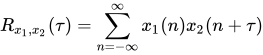
which defines the level of correlation between the outputs of two sensors ${\displaystyle x_{1}}$ and ${\displaystyle x_{2}}$. In general, a higher level of correlation means that the argument ${\displaystyle \tau }$ is relatively close to the actual time-difference-of-arrival. For two sensors next to each other the TDOA is given by

${\displaystyle \tau _{\text{true}}={\frac {d_{\text{spacing}}}{c}}}$

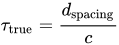
where ${\displaystyle c}$ is the speed of sound in the medium surrounding the sensors and the source.

A well-known example of TDOA is the interaural time difference. The interaural time difference is the difference in arrival time of a sound between two ears. The interaural time difference is given by

${\displaystyle \Delta t={\frac {x\cos \theta }{c}}}$

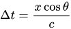
where

${\displaystyle \Delta t}$ is the time difference in seconds,

${\displaystyle x}$ is the distance between the two sensors (ears) in meters,

${\displaystyle \theta }$ is the angle between the baseline of the sensors (ears) and the incident sound, in degrees.

In trigonometry and geometry, triangulation is the process of determining the location of a point by measuring angles to it from known points at either end of a fixed baseline, rather than measuring distances to the point directly (trilateration). The point can then be fixed as the third point of a triangle with one known side and two known angles.

For acoustic localization this means that if the source direction is measured at two or more locations in space, it is possible to triangulate its location.

Steered response power (SRP) methods are a class of indirect acoustic source localization methods. Instead of estimating a set of time-differences of arrival (TDOAs) between pairs of microphones and combining the acquired estimates to find the source location, indirect methods search for a candidate source location over a grid of spatial points. In this context, methods such as the steered-response power with phase transform (SRP-PHAT)^[5] are usually interpreted as finding the candidate location that maximizes the output of a delay-and-sum beamformer. The method has been shown to be very robust to noise and reverberation, motivating the development of modified approaches aimed at increasing its performance in real-time acoustic processing applications.^[6]

Military uses have included locating submarines^[7] and aircraft.^[8] The first use of this type of equipment was claimed by Commander Alfred Rawlinson of the Royal Naval Volunteer Reserve, who in the autumn of 1916 was commanding a mobile anti-aircraft battery on the east coast of England. He needed a means of locating Zeppelins during cloudy conditions and improvised an apparatus from a pair of gramophone horns mounted on a rotating pole. Several of these equipments were able to give a fairly accurate fix on the approaching airships, allowing the guns to be directed at them despite being out of sight.^[9] Although no hits were obtained by this method, Rawlinson claimed to have forced a Zeppelin to jettison its bombs on one occasion.^[10]

The air-defense instruments usually consisted of large horns or microphones connected to the operators' ears using tubing, much like a very large stethoscope.^[11][12]

End of the 1920s, an operational comparison of multiple large acoustic listening devices from different nations by the Meetgebouw in The Netherlands showed drawbacks. Fundamental research showed that the human ear is better than one understood in the 20s and 30s. New listening devices closer to the ears and with airtight connections were developed. Moreover, mechanical prediction equipment, given the slow speed of sound as compared to the faster planes, and height corrections provided information to point the searchlight operators and the anti-aircraft gunners to where the detected aircraft flies. Searchlights and guns needed to be at a distance from the listening device. Therefore, electric direction indicator devices were developed.^[13]

Most of the work on anti-aircraft sound ranging was done by the British. They developed an extensive network of sound mirrors that were used from World War I through World War II.^[14][15] Sound mirrors normally work by using moveable microphones to find the angle that maximizes the amplitude of sound received, which is also the bearing angle to the target. Two sound mirrors at different positions will generate two different bearings, which allows the use of triangulation to determine a sound source's position.

As World War II neared, radar began to become a credible alternative to the sound location of aircraft. For typical aircraft speeds of that time, sound location only gave a few minutes of warning.^[8] The acoustic location stations were left in operation as a backup to radar, as exemplified during the Battle of Britain.^[16] Today, the abandoned sites are still in existence and are readily accessible.^{[14][dead link]}

After World War II, sound ranging played no further role in anti-aircraft operations.^{[citation needed][needs update]}

Active locators have some sort of signal generation device, in addition to a listening device. The two devices do not have to be located together.

Sonar (sound navigation and ranging) is a technique that uses sound propagation under water (or occasionally in air) to navigate, communicate or to detect other vessels. There are two kinds of sonar – active and passive. A single active sonar can localize in range and bearing as well as measuring radial speed. However, a single passive sonar can only localize in bearing directly, though Target Motion Analysis can be used to localize in range, given time. Multiple passive sonars can be used for range localization by triangulation or correlation, directly.

Dolphins, whales and bats use echolocation to detect prey and avoid obstacles.

Having speakers/ultrasonic transmitters emitting sound at known positions and time, the position of a target equipped with a microphone/ultrasonic receiver can be estimated based on the time of arrival of the sound. The accuracy is usually poor under non-line-of-sight conditions, where there are blockages in between the transmitters and the receivers. ^[17]

Seismic surveys involve the generation of sound waves to measure underground structures. Source waves are generally created by percussion mechanisms located near the ground or water surface, typically dropped weights, vibroseis trucks, or explosives. Data are collected with geophones, then stored and processed by computer. Current technology allows the generation of 3D images of underground rock structures using such equipment.

Because the cost of the associated sensors and electronics is dropping, the use of sound ranging technology is becoming accessible for other uses, such as for locating wildlife.^[18]

• Acoustic camera
• 3D sound reconstruction
• 3D sound localization
• Sound localization
• Boomerang
• Multilateration
• Acoustic mirror
• Acoustic wayfinding, the practice of using auditory cues and sound markers to navigate indoor and outdoor spaces
• Animal echolocation, animals emitting sound and listening to the echo in order to locate objects or navigate
• Echo sounding, listening to the echo of sound pulses to measure the distance to the bottom of the sea, a special case of sonar
• Gunfire locator
• Human echolocation, the use of echolocation by blind people
• Human bycatch
• Medical ultrasonography, the use of ultrasound echoes to look inside the body
• Sensory substitution