Bode plot

Among his several important contributions to circuit theory and control theory, engineer Hendrik Wade Bode, while working at Bell Labs in the 1930s, devised a simple but accurate method for graphing gain and phase-shift plots. These bear his name, Bode gain plot and Bode phase plot. "Bode" is often pronounced in English as /ˈboʊdi/ BOH-dee, whereas in Dutch it is usually [ˈboːdə], closer to English /ˈboʊdə/ BOH-də, which is preferred by his family, but less common among researchers.^[2][3]

Bode was faced with the problem of designing stable amplifiers with feedback for use in telephone networks. He developed the graphical design technique of the Bode plots to show the gain margin and phase margin required to maintain stability under variations in circuit characteristics caused during manufacture or during operation.^[4] The principles developed were applied to design problems of servomechanisms and other feedback control systems. The Bode plot is an example of analysis in the frequency domain.

The Bode plot for a linear, time-invariant system with transfer function ${\displaystyle H(s)}$ (${\displaystyle s}$ being the complex frequency in the Laplace domain) consists of a magnitude plot and a phase plot.

The Bode magnitude plot is the graph of the function ${\displaystyle |H(s=j\omega )|}$ of frequency ${\displaystyle \omega }$ (with ${\displaystyle j}$ being the imaginary unit). The ${\displaystyle \omega }$-axis of the magnitude plot is logarithmic and the magnitude is given in decibels, i.e., a value for the magnitude ${\displaystyle |H|}$ is plotted on the axis at ${\displaystyle 20\log _{10}|H|}$.

The Bode phase plot is the graph of the phase, commonly expressed in degrees, of the argument function ${\displaystyle \arg \left(H(s=j\omega )\right)}$ as a function of ${\displaystyle \omega }$. The phase is plotted on the same logarithmic ${\displaystyle \omega }$-axis as the magnitude plot, but the value for the phase is plotted on a linear vertical axis.

This section illustrates that a Bode plot is a visualization of the frequency response of a system.

Consider a linear, time-invariant system with transfer function ${\displaystyle H(s)}$. Assume that the system is subject to a sinusoidal input with frequency ${\displaystyle \omega }$,

${\displaystyle u(t)=\sin(\omega t),}$

that is applied persistently, i.e. from a time ${\displaystyle -\infty }$ to a time ${\displaystyle t}$. The response will be of the form

${\displaystyle y(t)=y_{0}\sin(\omega t+\varphi ),}$

i.e., also a sinusoidal signal with amplitude ${\displaystyle y_{0}}$ shifted by a phase ${\displaystyle \varphi }$ with respect to the input.

It can be shown^[5] that the magnitude of the response is

${\displaystyle y_{0}=|H(\mathrm {j} \omega )|}$

1

and that the phase shift is

${\displaystyle \varphi =\arg H(\mathrm {j} \omega ).}$

2

In summary, subjected to an input with frequency ${\displaystyle \omega }$, the system responds at the same frequency with an output that is amplified by a factor ${\displaystyle |H(\mathrm {j} \omega )|}$ and phase-shifted by ${\displaystyle \arg H(\mathrm {j} \omega )}$. These quantities, thus, characterize the frequency response and are shown in the Bode plot.

For many practical problems, the detailed Bode plots can be approximated with straight-line segments that are asymptotes of the precise response. The effect of each of the terms of a multiple element transfer function can be approximated by a set of straight lines on a Bode plot. This allows a graphical solution of the overall frequency response function. Before widespread availability of digital computers, graphical methods were extensively used to reduce the need for tedious calculation; a graphical solution could be used to identify feasible ranges of parameters for a new design.

The premise of a Bode plot is that one can consider the log of a function in the form

${\displaystyle f(x)=A\prod (x-c_{n})^{a_{n}}}$

as a sum of the logs of its zeros and poles:

${\displaystyle \log(f(x))=\log(A)+\sum a_{n}\log(x-c_{n}).}$

This idea is used explicitly in the method for drawing phase diagrams. The method for drawing amplitude plots implicitly uses this idea, but since the log of the amplitude of each pole or zero always starts at zero and only has one asymptote change (the straight lines), the method can be simplified.

Amplitude decibels is usually done using ${\displaystyle {\text{dB}}=20\log _{10}(X)}$ to define decibels. Given a transfer function in the form

${\displaystyle H(s)=A\prod {\frac {(s-x_{n})^{a_{n}}}{(s-y_{n})^{b_{n}}}},}$

where ${\displaystyle x_{n}}$ and ${\displaystyle y_{n}}$ are constants, ${\displaystyle s=\mathrm {j} \omega }$, ${\displaystyle a_{n},b_{n}>0}$, and ${\displaystyle H}$ is the transfer function:

• At every value of s where ${\displaystyle \omega =x_{n}}$ (a zero), increase the slope of the line by ${\displaystyle 20a_{n}\ {\text{dB}}}$ per decade.
• At every value of s where ${\displaystyle \omega =y_{n}}$ (a pole), decrease the slope of the line by ${\displaystyle 20b_{n}\ {\text{dB}}}$ per decade.
• The initial value of the graph depends on the boundaries. The initial point is found by putting the initial angular frequency ${\displaystyle \omega }$ into the function and finding ${\displaystyle |H(\mathrm {j} \omega )|}$.
• The initial slope of the function at the initial value depends on the number and order of zeros and poles that are at values below the initial value, and is found using the first two rules.

To handle irreducible 2nd-order polynomials, ${\displaystyle ax^{2}+bx+c}$ can, in many cases, be approximated as ${\displaystyle ({\sqrt {a}}x+{\sqrt {c}})^{2}}$.

Note that zeros and poles happen when ${\displaystyle \omega }$ is equal to a certain ${\displaystyle x_{n}}$ or ${\displaystyle y_{n}}$. This is because the function in question is the magnitude of ${\displaystyle H(\mathrm {j} \omega )}$, and since it is a complex function, ${\displaystyle |H(\mathrm {j} \omega )|={\sqrt {H\cdot H^{*}}}}$. Thus at any place where there is a zero or pole involving the term ${\displaystyle (s+x_{n})}$, the magnitude of that term is ${\displaystyle {\sqrt {(x_{n}+\mathrm {j} \omega )(x_{n}-\mathrm {j} \omega )}}={\sqrt {x_{n}^{2}+\omega ^{2}}}}$.

To correct a straight-line amplitude plot:

• At every zero, put a point ${\displaystyle 3a_{n}\ {\text{dB}}}$ above the line.
• At every pole, put a point ${\displaystyle 3b_{n}\ {\text{dB}}}$ below the line.
• Draw a smooth curve through those points using the straight lines as asymptotes (lines which the curve approaches).

Note that this correction method does not incorporate how to handle complex values of ${\displaystyle x_{n}}$ or ${\displaystyle y_{n}}$. In the case of an irreducible polynomial, the best way to correct the plot is to actually calculate the magnitude of the transfer function at the pole or zero corresponding to the irreducible polynomial, and put that dot over or under the line at that pole or zero.

Given a transfer function in the same form as above,

${\displaystyle H(s)=A\prod {\frac {(s-x_{n})^{a_{n}}}{(s-y_{n})^{b_{n}}}},}$

the idea is to draw separate plots for each pole and zero, then add them up. The actual phase curve is given by

${\displaystyle \varphi (s)=-\arctan {\frac {\operatorname {Im} [H(s)]}{\operatorname {Re} [H(s)]}}.}$

To draw the phase plot, for each pole and zero:

• If ${\displaystyle A}$ is positive, start line (with zero slope) at 0°.
• If ${\displaystyle A}$ is negative, start line (with zero slope) at −180°.
• If the sum of the number of unstable zeros and poles is odd, add 180° to that basis.
• At every ${\displaystyle \omega =|x_{n}|}$ (for stable zeros ${\displaystyle -\operatorname {Re} (z)<0}$), increase the slope by ${\displaystyle 45a_{n}}$ degrees per decade, beginning one decade before ${\displaystyle \omega =|x_{n}|}$ (e.g., ${\displaystyle |x_{n}|/10}$).
• At every ${\displaystyle \omega =|y_{n}|}$ (for stable poles ${\displaystyle -\operatorname {Re} (p)<0}$), decrease the slope by ${\displaystyle 45b_{n}}$ degrees per decade, beginning one decade before ${\displaystyle \omega =|y_{n}|}$ (e.g., ${\displaystyle |y_{n}|/10}$).
• "Unstable" (right half-plane) poles and zeros (${\displaystyle \operatorname {Re} (s)>0}$) have opposite behavior.
• Flatten the slope again when the phase has changed by ${\displaystyle 90a_{n}}$ degrees (for a zero) or ${\displaystyle 90b_{n}}$ degrees (for a pole).
• After plotting one line for each pole or zero, add the lines together to obtain the final phase plot; that is, the final phase plot is the superposition of each earlier phase plot.

To create a straight-line plot for a first-order (one-pole) low-pass filter, one considers the normalized form of the transfer function in terms of the angular frequency:

${\displaystyle H_{\text{lp}}(\mathrm {j} \omega )={\frac {1}{1+\mathrm {j} {\frac {\omega }{\omega _{\text{c}}}}}}.}$

The Bode plot is shown in Figure 1(b) above, and construction of the straight-line approximation is discussed next.

The magnitude (in decibels) of the transfer function above (normalized and converted to angular-frequency form), given by the decibel gain expression ${\displaystyle A_{\text{vdB}}}$:

${\displaystyle {\begin{aligned}A_{\text{vdB}}&=20\log |H_{\text{lp}}(\mathrm {j} \omega )|\\&=20\log {\frac {1}{\left|1+\mathrm {j} {\frac {\omega }{\omega _{\text{c}}}}\right|}}\\&=-20\log \left|1+\mathrm {j} {\frac {\omega }{\omega _{\text{c}}}}\right|\\&=-10\log \left(1+{\frac {\omega ^{2}}{\omega _{\text{c}}^{2}}}\right).\end{aligned}}}$

Then plotted versus input frequency ${\displaystyle \omega }$ on a logarithmic scale, can be approximated by two lines, forming the asymptotic (approximate) magnitude Bode plot of the transfer function:

• The first line for angular frequencies below ${\displaystyle \omega _{\text{c}}}$ is a horizontal line at 0 dB, since at low frequencies the ${\displaystyle \omega /\omega _{\text{c}}}$ term is small and can be neglected, making the decibel gain equation above equal to zero.
• The second line for angular frequencies above ${\displaystyle \omega _{\text{c}}}$ is a line with a slope of −20 dB per decade, since at high frequencies the ${\displaystyle \omega /\omega _{\text{c}}}$ term dominates, and the decibel gain expression above simplifies to ${\displaystyle -20\log(\omega /\omega _{\text{c}})}$, which is a straight line with a slope of −20 dB per decade.

These two lines meet at the corner frequency ${\displaystyle \omega _{\text{c}}}$. From the plot, it can be seen that for frequencies well below the corner frequency, the circuit has an attenuation of 0 dB, corresponding to a unity pass-band gain, i.e. the amplitude of the filter output equals the amplitude of the input. Frequencies above the corner frequency are attenuated – the higher the frequency, the higher the attenuation.

The phase Bode plot is obtained by plotting the phase angle of the transfer function given by

${\displaystyle \arg H_{\text{lp}}(\mathrm {j} \omega )=-\tan ^{-1}{\frac {\omega }{\omega _{\text{c}}}}}$

versus ${\displaystyle \omega }$, where ${\displaystyle \omega }$ and ${\displaystyle \omega _{\text{c}}}$ are the input and cutoff angular frequencies respectively. For input frequencies much lower than corner, the ratio ${\displaystyle \omega /\omega _{\text{c}}}$ is small, and therefore the phase angle is close to zero. As the ratio increases, the absolute value of the phase increases and becomes −45° when ${\displaystyle \omega =\omega _{\text{c}}}$. As the ratio increases for input frequencies much greater than the corner frequency, the phase angle asymptotically approaches −90°. The frequency scale for the phase plot is logarithmic.

The horizontal frequency axis, in both the magnitude and phase plots, can be replaced by the normalized (nondimensional) frequency ratio ${\displaystyle \omega /\omega _{\text{c}}}$. In such a case the plot is said to be normalized, and units of the frequencies are no longer used, since all input frequencies are now expressed as multiples of the cutoff frequency ${\displaystyle \omega _{\text{c}}}$.

Figures 2–5 further illustrate construction of Bode plots. This example with both a pole and a zero shows how to use superposition. To begin, the components are presented separately.

Figure 2 shows the Bode magnitude plot for a zero and a low-pass pole, and compares the two with the Bode straight line plots. The straight-line plots are horizontal up to the pole (zero) location and then drop (rise) at 20 dB/decade. The second Figure 3 does the same for the phase. The phase plots are horizontal up to a frequency factor of ten below the pole (zero) location and then drop (rise) at 45°/decade until the frequency is ten times higher than the pole (zero) location. The plots then are again horizontal at higher frequencies at a final, total phase change of 90°.

Figure 4 and Figure 5 show how superposition (simple addition) of a pole and zero plot is done. The Bode straight line plots again are compared with the exact plots. The zero has been moved to higher frequency than the pole to make a more interesting example. Notice in Figure 4 that the 20 dB/decade drop of the pole is arrested by the 20 dB/decade rise of the zero resulting in a horizontal magnitude plot for frequencies above the zero location. Notice in Figure 5 in the phase plot that the straight-line approximation is pretty approximate in the region where both pole and zero affect the phase. Notice also in Figure 5 that the range of frequencies where the phase changes in the straight line plot is limited to frequencies a factor of ten above and below the pole (zero) location. Where the phase of the pole and the zero both are present, the straight-line phase plot is horizontal because the 45°/decade drop of the pole is arrested by the overlapping 45°/decade rise of the zero in the limited range of frequencies where both are active contributors to the phase.

• Example with pole and zero
• 
  Figure 2: Bode magnitude plot for zero and low-pass pole; curves labeled "Bode" are the straight-line Bode plots
• 
  Figure 3: Bode phase plot for zero and low-pass pole; curves labeled "Bode" are the straight-line Bode plots
• 
  Figure 4: Bode magnitude plot for pole-zero combination; the location of the zero is ten times higher than in Figures 2 and 3; curves labeled "Bode" are the straight-line Bode plots
• 
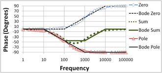  Figure 5: Bode phase plot for pole-zero combination; the location of the zero is ten times higher than in Figures 2 and 3; curves labeled "Bode" are the straight-line Bode plots

Bode plots are used to assess the stability of negative-feedback amplifiers by finding the gain and phase margins of an amplifier. The notion of gain and phase margin is based upon the gain expression for a negative feedback amplifier given by

${\displaystyle A_{\text{FB}}={\frac {A_{\text{OL}}}{1+\beta A_{\text{OL}}}},}$

where A_FB is the gain of the amplifier with feedback (the closed-loop gain), β is the feedback factor, and A_OL is the gain without feedback (the open-loop gain). The gain A_OL is a complex function of frequency, with both magnitude and phase.^{[note 1]} Examination of this relation shows the possibility of infinite gain (interpreted as instability) if the product βA_OL = −1 (that is, the magnitude of βA_OL is unity and its phase is −180°, the so-called Barkhausen stability criterion). Bode plots are used to determine just how close an amplifier comes to satisfying this condition.

Key to this determination are two frequencies. The first, labeled here as f₁₈₀, is the frequency where the open-loop gain flips sign. The second, labeled here f_0 dB, is the frequency where the magnitude of the product |βA_OL| = 1 = 0 dB. That is, frequency f₁₈₀ is determined by the condition

${\displaystyle \beta A_{\text{OL}}(f_{180})=-|\beta A_{\text{OL}}(f_{180})|=-|\beta A_{\text{OL}}|_{180},}$

where vertical bars denote the magnitude of a complex number, and frequency f_0 dB is determined by the condition

${\displaystyle |\beta A_{\text{OL}}(f_{\text{0 dB}})|=1.}$

One measure of proximity to instability is the gain margin. The Bode phase plot locates the frequency where the phase of βA_OL reaches −180°, denoted here as frequency f₁₈₀. Using this frequency, the Bode magnitude plot finds the magnitude of βA_OL. If |βA_OL|₁₈₀ ≥ 1, the amplifier is unstable, as mentioned. If |βA_OL|₁₈₀ < 1, instability does not occur, and the separation in dB of the magnitude of |βA_OL|₁₈₀ from |βA_OL| = 1 is called the gain margin. Because a magnitude of 1 is 0 dB, the gain margin is simply one of the equivalent forms: ${\displaystyle 20\log _{10}|\beta A_{\text{OL}}|_{180}=20\log _{10}|A_{\text{OL}}|-20\log _{10}\beta ^{-1}}$.

Another equivalent measure of proximity to instability is the phase margin. The Bode magnitude plot locates the frequency where the magnitude of |βA_OL| reaches unity, denoted here as frequency f_0 dB. Using this frequency, the Bode phase plot finds the phase of βA_OL. If the phase of βA_OL(f_0 dB) > −180°, the instability condition cannot be met at any frequency (because its magnitude is going to be < 1 when f = f₁₈₀), and the distance of the phase at f_0 dB in degrees above −180° is called the phase margin.

If a simple yes or no on the stability issue is all that is needed, the amplifier is stable if f_0 dB < f₁₈₀. This criterion is sufficient to predict stability only for amplifiers satisfying some restrictions on their pole and zero positions (minimum phase systems). Although these restrictions usually are met, if they are not, then another method must be used, such as the Nyquist plot.^[6][7] Optimal gain and phase margins may be computed using Nevanlinna–Pick interpolation theory.^[8]

Figures 6 and 7 illustrate the gain behavior and terminology. For a three-pole amplifier, Figure 6 compares the Bode plot for the gain without feedback (the open-loop gain) A_OL with the gain with feedback A_FB (the closed-loop gain). See negative feedback amplifier for more detail.

In this example, A_OL = 100 dB at low frequencies, and 1 / β = 58 dB. At low frequencies, A_FB ≈ 58 dB as well.

Because the open-loop gain A_OL is plotted and not the product β A_OL, the condition A_OL = 1 / β decides f_0 dB. The feedback gain at low frequencies and for large A_OL is A_FB ≈ 1 / β (look at the formula for the feedback gain at the beginning of this section for the case of large gain A_OL), so an equivalent way to find f_0 dB is to look where the feedback gain intersects the open-loop gain. (Frequency f_0 dB is needed later to find the phase margin.)

Near this crossover of the two gains at f_0 dB, the Barkhausen criteria are almost satisfied in this example, and the feedback amplifier exhibits a massive peak in gain (it would be infinity if β A_OL = −1). Beyond the unity gain frequency f_0 dB, the open-loop gain is sufficiently small that A_FB ≈ A_OL (examine the formula at the beginning of this section for the case of small A_OL).

Figure 7 shows the corresponding phase comparison: the phase of the feedback amplifier is nearly zero out to the frequency f₁₈₀ where the open-loop gain has a phase of −180°. In this vicinity, the phase of the feedback amplifier plunges abruptly downward to become almost the same as the phase of the open-loop amplifier. (Recall, A_FB ≈ A_OL for small A_OL.)

Comparing the labeled points in Figure 6 and Figure 7, it is seen that the unity gain frequency f_0 dB and the phase-flip frequency f₁₈₀ are very nearly equal in this amplifier, f₁₈₀ ≈ f_0 dB ≈ 3.332 kHz, which means the gain margin and phase margin are nearly zero. The amplifier is borderline stable.

Figures 8 and 9 illustrate the gain margin and phase margin for a different amount of feedback β. The feedback factor is chosen smaller than in Figure 6 or 7, moving the condition | β A_OL | = 1 to lower frequency. In this example, 1 / β = 77 dB, and at low frequencies A_FB ≈ 77 dB as well.

Figure 8 shows the gain plot. From Figure 8, the intersection of 1 / β and A_OL occurs at f_0 dB = 1 kHz. Notice that the peak in the gain A_FB near f_0 dB is almost gone.^{[note 2][9]}

Figure 9 is the phase plot. Using the value of f_0 dB = 1 kHz found above from the magnitude plot of Figure 8, the open-loop phase at f_0 dB is −135°, which is a phase margin of 45° above −180°.

Using Figure 9, for a phase of −180° the value of f₁₈₀ = 3.332 kHz (the same result as found earlier, of course^{[note 3]}). The open-loop gain from Figure 8 at f₁₈₀ is 58 dB, and 1 / β = 77 dB, so the gain margin is 19 dB.

Stability is not the sole criterion for amplifier response, and in many applications a more stringent demand than stability is good step response. As a rule of thumb, good step response requires a phase margin of at least 45°, and often a margin of over 70° is advocated, particularly where component variation due to manufacturing tolerances is an issue.^[9] See also the discussion of phase margin in the step response article.

• Examples
• 
  Figure 6: Gain of feedback amplifier A_FB in dB and corresponding open-loop amplifier A_OL. Parameter 1/β = 58 dB, and at low frequencies A_FB ≈ 58 dB as well. The gain margin in this amplifier is nearly zero because | βA_OL| = 1 occurs at almost f = f_180°.
• 
  Figure 7: Phase of feedback amplifier °A_FB in degrees and corresponding open-loop amplifier °A_OL. The phase margin in this amplifier is nearly zero because the phase-flip occurs at almost the unity gain frequency f = f_0 dB where | βA_OL| = 1.
• 
  Figure 8: Gain of feedback amplifier A_FB in dB and corresponding open-loop amplifier A_OL. In this example, 1 / β = 77 dB. The gain margin in this amplifier is 19 dB.
• 
  Figure 9: Phase of feedback amplifier A_FB in degrees and corresponding open-loop amplifier A_OL. The phase margin in this amplifier is 45°.

The Bode plotter is an electronic instrument resembling an oscilloscope, which produces a Bode diagram, or a graph, of a circuit's voltage gain or phase shift plotted against frequency in a feedback control system or a filter. An example of this is shown in Figure 10. It is extremely useful for analyzing and testing filters and the stability of feedback control systems, through the measurement of corner (cutoff) frequencies and gain and phase margins.

This is identical to the function performed by a vector network analyzer, but the network analyzer is typically used at much higher frequencies.

For education and research purposes, plotting Bode diagrams for given transfer functions facilitates better understanding and getting faster results (see external links).

Two related plots that display the same data in different coordinate systems are the Nyquist plot and the Nichols plot. These are parametric plots, with frequency as the input and magnitude and phase of the frequency response as the output. The Nyquist plot displays these in polar coordinates, with magnitude mapping to radius and phase to argument (angle). The Nichols plot displays these in rectangular coordinates, on the log scale.

• 
  Figure 11: A Nyquist plot.
• 
  Figure 12: A Nichols plot of the same response from Figure 11.

• Analog signal processing
• Phase margin
• Bode's sensitivity integral
• Bode's magnitude (gain)–phase relation
• Dielectric spectroscopy

References

[edit]- ^ R. K. Rao Yarlagadda (2010). Analog and Digital Signals and Systems. Springer Science & Business Media. p. 243. ISBN 978-1-4419-0034-0.
- ^ Van Valkenburg, M. E. University of Illinois at Urbana-Champaign, "In memoriam: Hendrik W. Bode (1905-1982)", IEEE Transactions on Automatic Control, Vol. AC-29, No 3., March 1984, pp. 193–194. Quote: "Something should be said about his name. To his colleagues at Bell Laboratories and the generations of engineers that have followed, the pronunciation is boh-dee. The Bode family preferred that the original Dutch be used as boh-dah."
- ^ "Vertaling van postbode, NL>EN". mijnwoordenboek.nl. Retrieved 2013-10-07.
- ^ David A. Mindell Between Human and Machine: Feedback, Control, and Computing Before Cybernetics JHU Press, 2004, ISBN 0801880572, pp. 127–131.
- ^ Skogestad, Sigurd; Postlewaite, Ian (2005). Multivariable Feedback Control. Chichester, West Sussex, England: John Wiley & Sons, Ltd. ISBN 0-470-01167-X.
- ^ Thomas H. Lee (2004). "§14.6. Gain and Phase Margins as Stability Measures". The design of CMOS radio-frequency integrated circuits (2nd ed.). Cambridge UK: Cambridge University Press. pp. 451–453. ISBN 0-521-83539-9.
- ^ William S. Levine (1996). "§10.1. Specifications of Control System". The control handbook: the electrical engineering handbook series (2nd ed.). Boca Raton FL: CRC Press/IEEE Press. p. 163. ISBN 0-8493-8570-9.
- ^ Allen Tannenbaum (February 1981). Invariance and Systems Theory: Algebraic and Geometric Aspects. New York, NY: Springer-Verlag. ISBN 9783540105657.
- ^ a b Willy M C Sansen (2006). Analog design essentials. Dordrecht, The Netherlands: Springer. pp. 157–163. ISBN 0-387-25746-2.
External links
[edit]- How to draw piecewise asymptotic Bode plots
- Gnuplot code for generating Bode plot: DIN-A4 printing template (pdf)
Bode plot
View on GrokipediaIntroduction
Overview
A Bode plot is a graphical tool used to represent the frequency response of linear time-invariant (LTI) systems, typically presented as a pair of semi-logarithmic graphs: one plotting the magnitude response in decibels (dB) against the logarithm of angular frequency (rad/s), and the other plotting the phase response in degrees against the same logarithmic frequency scale.[9][6] The primary purpose of Bode plots is to provide a visual assessment of how a system's transfer function behaves across frequencies, highlighting variations in gain (amplification or attenuation) and phase shift, which are essential for applications in control systems engineering, signal processing, and analog circuit design.[10][6] This frequency-domain representation simplifies the identification of key system properties without requiring full-time-domain simulations. Originating from the work of Hendrik Wade Bode at Bell Laboratories in the 1930s, the plot leverages logarithmic scales to accommodate wide frequency ranges effectively. Major advantages include the ability to sketch approximate plots by hand using straight-line asymptotes, offering rapid insights into bandwidth limitations, resonant frequencies, and stability criteria such as gain and phase margins.[2]Historical Development
The Bode plot was developed by Hendrik Wade Bode during the early 1930s while he was employed as a mathematician at Bell Laboratories, where he focused on advancing the design of feedback amplifiers for improved performance in communication systems. Bode's approach emphasized graphical representations of frequency response using asymptotic approximations, which simplified the analysis of complex networks compared to earlier numerical methods. This work built upon foundational frequency response concepts introduced by Harry Nyquist in the 1920s, particularly his 1932 paper on regeneration theory, which analyzed stability in feedback systems through contour plots but lacked the semi-logarithmic scaling that Bode later refined for practical engineering use. In the context of early feedback amplifier design, Bode's techniques addressed challenges in maintaining stability and gain under varying conditions, which were critical for long-distance telephony at Bell Labs. During World War II, these methods supported the rapid development of reliable communications and radar systems, as feedback amplifiers became essential for military electronics.[11] Bode formalized his graphical method in the 1945 book Network Analysis and Feedback Amplifier Design, which integrated network theory with feedback principles and introduced the plots as a standard tool for visualizing magnitude and phase responses. By the 1950s, Bode plots had evolved into a cornerstone of control theory, widely adopted alongside Nyquist and root-locus methods for system design in academia and industry. The plots gained broad adoption in aerospace for flight control systems, in electronics for amplifier and filter design, and later in digital signal processing for analyzing discrete-time filters, reflecting their versatility across analog and digital domains. Additionally, Bode contributed key stability criteria, including gain and phase margins derived from the plots, which quantify a system's robustness to parameter variations and remain fundamental to feedback design.Mathematical Foundations
Definition and Notation
A Bode plot provides a graphical representation of the frequency response of a linear time-invariant (LTI) system, typically consisting of two separate graphs plotted against the logarithm of the angular frequency, . The magnitude plot displays the gain of the system in decibels (dB) as , where denotes the system's transfer function in the Laplace domain and the frequency response is given by upon substituting .[12][13] The phase plot shows the argument of the frequency response, , usually in degrees, illustrating the phase shift introduced by the system at each frequency .[14][15] The use of the decibel scale for the magnitude plot compresses the typically wide dynamic range of into a more manageable linear scale on a semilogarithmic graph, facilitating the analysis of systems with gains spanning multiple orders of magnitude.[13] Angular frequency is conventionally expressed in radians per second (rad/s), though plots may sometimes use frequency in hertz (Hz) by plotting against where ; phase angles are standardly in degrees but can be in radians for certain applications.[12][16] Bode plots are defined under the assumption of LTI systems, where the transfer function fully characterizes the steady-state response to sinusoidal inputs, enabling the frequency response to capture both amplitude and phase variations without time-varying or nonlinear effects.[15][17] For minimum-phase systems—those with all zeros and poles in the left-half s-plane—the phase plot can be uniquely related to the magnitude plot via the Hilbert transform, though the general definition applies to stable LTI systems regardless of phase minimality.[18] In standard notation, key features such as corner frequencies (or breakpoints) mark the values of where the transfer function's poles or zeros occur, corresponding to changes in the slope of the asymptotic magnitude plot by dB per decade for simple poles/zeros.[14] This notation emphasizes the logarithmic scales to highlight multiplicative effects of poles and zeros on the overall response.[12]Transfer Function in Frequency Domain
The frequency response of a linear time-invariant system is obtained by evaluating its transfer function along the imaginary axis of the complex plane, where and is the angular frequency in radians per second. This substitution transforms the Laplace-domain transfer function into the frequency-domain form , which describes the system's steady-state response to sinusoidal inputs of frequency . For a general transfer function , where and are the numerator and denominator polynomials, respectively, the frequency response becomes . This approach is fundamental in control systems analysis, as detailed in standard engineering references.[19][15] The magnitude of the frequency response is given by , where and denote the real and imaginary parts of the complex-valued . The corresponding phase angle is , which measures the phase shift introduced by the system. These expressions arise directly from the properties of complex numbers and enable the separation of amplitude and phase effects in Bode plot construction.[19][20] In pole-zero form, the transfer function is expressed as , where is the gain constant, are the zeros, and are the poles. Substituting yields , and the magnitude simplifies to . Geometrically, this represents the product of the distances from the point in the complex plane to each zero divided by the distances to each pole, scaled by , providing an intuitive basis for understanding frequency-dependent behavior.[21][22] At low frequencies (), the magnitude approaches a constant value equal to if there are no poles or zeros at the origin, reflecting the system's DC gain determined by the pole-zero configuration. Conversely, at high frequencies (), the behavior depends on the relative order of poles and zeros: if the number of poles exceeds the number of zeros by , then (product of leading coefficients), leading to a roll-off proportional to ; equal orders yield a constant asymptote scaled by the ratio of leading coefficients. These asymptotic limits establish the foundational slopes and levels for Bode magnitude plots, often expressed in decibels for logarithmic scaling.[21][22]Construction Methods
Asymptotic Amplitude Plot
The asymptotic amplitude plot provides a straight-line approximation to the magnitude response of a system's transfer function, expressed in decibels (dB) versus the base-10 logarithm of angular frequency (rad/s). This method facilitates rapid hand-sketching of the frequency response by representing the exact magnitude curve with piecewise linear segments that capture the dominant behavior across frequency decades. Developed by Hendrik W. Bode, the approximation emphasizes the locations of poles and zeros to determine changes in slope, enabling engineers to assess gain variations without detailed computation.[21] For a transfer function normalized to have a DC gain of unity (0 dB), the low-frequency portion of the plot is a horizontal straight line at 0 dB, extending until the first corner frequency. The corner frequency for a real zero at (where ) or a real pole at (where ) is given by or , respectively, marking the point where the slope changes. At each such corner frequency, the asymptotic slope increases by +20 dB/decade for a zero and decreases by -20 dB/decade for a pole.[21][23] When multiple poles or zeros occur, their effects on the slope are additive; for instance, a double pole at the same location results in a total slope change of -40 dB/decade starting at its corner frequency. Higher-order factors, such as quadratic terms from complex conjugate poles, contribute slope changes proportional to their multiplicity (e.g., -40 dB/decade for a pair of complex poles). The initial slope before any corner frequencies is typically 0 dB/decade for normalized systems without poles or zeros at the origin, and subsequent segments are drawn by cumulatively adjusting the slope at each ordered corner frequency.[24][25] Normalization to the DC gain ensures the low-frequency asymptote aligns at 0 dB, simplifying comparisons across systems, while the logarithmic frequency scale (with in rad/s) highlights the decade-wise behavior and multiplicative nature of frequency responses. Corner frequencies are directly identified from the pole-zero plot in the s-plane, with the magnitude of each pole or zero location dictating the transition point. This approach approximates the exact magnitude , which involves products over pole and zero terms, by neglecting the gradual roll-off near corners for conceptual clarity.[21][22]Asymptotic Phase Plot
The asymptotic phase plot in a Bode diagram approximates the phase angle ∠H(jω) of a system's transfer function H(s) using straight-line segments on a semi-logarithmic frequency scale, facilitating quick estimation of frequency response characteristics. This method decomposes the transfer function into its pole and zero factors, approximates each factor's phase contribution individually, and graphically sums them to obtain the overall phase behavior. The approximation is particularly useful for hand-sketching and initial design analysis in control systems.[21] For a real zero with corner frequency ω_z, the phase contribution is 0° at low frequencies (ω ≪ ω_z), where the factor behaves as a constant. The phase then ramps upward at +45° per decade starting one decade before ω_z (at 0.1ω_z), reaches +45° at ω_z, and continues the linear increase to +90° one decade after (at 10ω_z), remaining constant at high frequencies (ω ≫ ω_z). Conversely, a real pole at corner frequency ω_p contributes 0° at low frequencies, a downward ramp at -45° per decade from 0.1ω_p to 10ω_p (passing through -45° at ω_p), and asymptotes to -90° at high frequencies. These ramps represent the piecewise linear approximation to the exact arctangent phase response of each factor.[21][26] The straight-line segments form horizontal lines at low and high frequencies, reflecting constant phase values (typically multiples of ±90° based on the net number of poles and zeros), connected by the linear ramps over the two-decade transition regions centered at each corner frequency. The total asymptotic phase plot is the graphical sum of all individual contributions, preserving additivity since phase angles add in the logarithmic domain. This summation can yield phase angles outside ±90° for systems with multiple elements, such as approaching -180° for two poles.[21][27] For complex conjugate poles or zeros, the asymptotic phase approximation adjusts the ramp characteristics according to the damping ratio ζ, with the total phase shift still being ±180° but concentrated over a frequency range influenced by ζ. Low damping (small ζ) results in a steeper transition near the natural frequency, while higher damping broadens it toward the real pole/zero behavior; however, the basic construction prioritizes real poles and zeros for straightforward approximations before incorporating these refinements.[21][26]Refinements and Corrections
While the asymptotic approximations provide a quick sketch of a Bode plot, refinements are necessary to capture the actual frequency response more accurately, particularly for hand-drawn diagrams. For the amplitude plot, the true magnitude curve deviates from the straight-line asymptotes near corner frequencies. Specifically, for a single real pole or zero, the actual magnitude |H(jω)| at the corner frequency ω_c is 3 dB above (for a zero) or below (for a pole) the asymptotic value, due to the factor of 1/√2 in the exact expression √(1 + (ω/ω_c)^2).[28] Phase refinements similarly adjust the abrupt asymptotic transitions to reflect the smooth variation in the actual phase response. For a single real pole, the exact phase is -arctan(ω/ω_c), starting at 0° for ω ≪ ω_c and gradually approaching -90° for ω ≫ ω_c, rather than jumping discontinuously at ω_c. A zero contributes +arctan(ω/ω_c), symmetrically smoothing toward +90°. These arctangent functions ensure the phase changes continuously over approximately two decades centered on the corner frequency.[21] For systems with underdamped complex conjugate poles, the amplitude plot exhibits a resonant peak not captured by the -40 dB/decade asymptote. The peak magnitude occurs at frequency ω_r = ω_n √(1 - 2ζ²), where ω_n is the natural frequency and ζ is the damping ratio, provided ζ < 1/√2 ≈ 0.707 to ensure a pronounced bump. The peak value is M_p = 1 / (2ζ √(1 - ζ²)), highlighting the system's oscillatory tendency; for ζ ≥ 1/√2, the response is maximally flat with no overshoot.[29] To incorporate these refinements in hand sketching, engineers calculate and plot exact |H(jω)| and phase values at critical frequencies—such as the corner frequency ω_c, one decade below and above it, and other decade-spaced points—then interpolate smoothly between them. This selective computation, often using the transfer function evaluated along the jω axis, bridges the gap between crude asymptotes and precise curves without requiring full numerical simulation.[30]Illustrative Examples
Single-Pole System
A single-pole system provides a fundamental example for illustrating Bode plot construction, particularly for a first-order low-pass filter with the transfer function , where is the cutoff angular frequency.[31] For simplicity, consider rad/s, normalizing the frequency axis such that the corner frequency aligns at 1 rad/s.[27] This transfer function represents the frequency response , enabling the derivation of magnitude and phase plots.[21] The magnitude plot, expressed in decibels as , features asymptotic behavior that is flat at 0 dB for , indicating unity gain in the low-frequency passband.[21] Beyond the corner frequency, for , the asymptote decreases at a rate of -20 dB per decade, characteristic of a single real pole contributing a first-order roll-off.[31] The actual magnitude curve smoothly transitions near , reaching exactly -3 dB at this point, where .[32] The phase plot, given by , starts at 0° for and asymptotically approaches -90° for , reflecting the progressive phase lag introduced by the pole.[21] At the corner frequency , the phase is precisely -45°.[31] In filter applications, the -20 dB/decade roll-off attenuates high-frequency components, suppressing noise while preserving low-frequency signals, whereas the phase lag can affect system timing and transient response.[32] To hand-sketch these plots, apply the general asymptotic construction rules: draw the magnitude asymptotes intersecting at 0 dB and on a logarithmic frequency axis (base-10 decades), then smooth the curve to pass through -3 dB at ; for phase, sketch straight-line approximations from 0° to -90° with a breakpoint decade before and after , adjusting to -45° at for the actual curve.[21] Exact points along the curves, such as magnitude at approximating 0 dB or phase at nearing -84.3°, can be computed directly from the expressions to refine the sketch.[27]System with Zero and Pole
A lead compensator, which introduces a zero and a pole in the transfer function, is commonly used to improve the phase margin in control systems by providing phase lead at specific frequencies. The transfer function for such a system is given by where are the zero and pole frequencies, respectively. For illustration, consider rad/s and rad/s, yielding a separation factor . This form ensures the zero dominates at lower frequencies, advancing the phase relative to a pole-only system.[33] In the Bode magnitude plot, the response remains flat at 0 dB for , then increases with a slope of +20 dB/decade between and , providing a high-frequency boost before flattening again for . The total boost in this region is dB, or approximately 20 dB for the example case, with the peak magnitude occurring near the geometric mean rad/s. This contrasts with a single-pole system, where the magnitude rolls off at -20 dB/decade without such enhancement.[34] The Bode phase plot starts at 0° for low frequencies, rises to a maximum lead of approximately , which evaluates to about +55° at , and then returns to 0° at high frequencies. The phase advance, peaking between and , enables better transient response in feedback loops compared to the lagging phase of a pole-only configuration.[33][34]Applications
Gain and Phase Margins
In control systems analysis, the gain margin (GM) quantifies the amount by which the gain of the open-loop transfer function can be increased before the closed-loop system becomes unstable. It is defined as , where is the phase crossover frequency at which the phase angle . Expressed in decibels, this becomes . If no such phase crossover exists, the gain margin is infinite, indicating inherent stability regardless of gain variations.[35][36] The phase margin (PM) measures the additional phase lag required at the gain crossover frequency to drive the system to instability. It is given by , where is the gain crossover frequency satisfying (or 0 dB on the Bode magnitude plot). These margins are extracted directly from the Bode plot: the gain margin from the magnitude at the phase crossover, and the phase margin from the phase at the gain crossover.[35][37] For robust stability in practical systems, a gain margin exceeding 6 dB and a phase margin greater than 45° are generally recommended, as these thresholds provide sufficient tolerance against parameter uncertainties and unmodeled dynamics while ensuring acceptable transient performance.[38][39] These values stem from empirical guidelines in frequency-domain design, balancing stability with responsiveness.[40] Gain and phase margins relate to the Nyquist stability criterion by assessing the proximity of the open-loop frequency response to the critical point (-1, 0) in the complex plane; larger margins correspond to greater distances from this point, reducing the risk of encirclement and instability.[41] In cases of conditional stability, where the Bode plot exhibits multiple gain or phase crossovers—often due to non-minimum phase zeros or complex pole structures—simple margin values may be misleading, necessitating full encirclement checks via the Nyquist plot to confirm stability across gain variations.[42]Stability Assessment
Bode plots provide a practical method for evaluating the stability of feedback control systems by examining the open-loop frequency response characteristics. The procedure begins by identifying key frequencies: the gain crossover frequency , where the magnitude plot intersects the 0 dB line, and the phase crossover frequency , where the phase plot reaches -180°. Gain and phase margins are then computed at these points, as detailed in the Gain and Phase Margins section, to quantify the distance from instability. Beyond margins, the slope of the magnitude plot at is critical; an ideal roll-off of -20 dB/decade suggests robust relative stability, as steeper slopes (e.g., -40 dB/decade or more) can amplify phase variations and promote oscillatory closed-loop behavior.[43] The gain crossover frequency also approximates the closed-loop system's bandwidth, particularly for designs with sufficient phase margins, enabling predictions of the frequency range over which the system responds effectively to inputs. Resonance in the closed-loop response can be assessed by deriving the complementary sensitivity function magnitude from the open-loop Bode plot; a peak exceeding 3 dB near signals underdamped dynamics and potential ringing in transients.[35][44] Bode plot analysis assumes minimum-phase systems, where phase shifts are uniquely determined by the magnitude response via the Bode gain-phase relationship. For non-minimum-phase systems featuring right-half-plane zeros, this assumption fails, leading to incomplete stability insights; such cases may exhibit inverse responses or bandwidth limitations, necessitating alternative tools like Nyquist plots for accurate encirclement checks.[45] In an example workflow, consider a system's Bode plot with rad/s and a phase margin exceeding 60° at that frequency. This configuration typically yields a damping ratio , ensuring a transient response with overshoot below 20% and settling time under 4/, indicative of stable, non-oscillatory performance.[46]Computational Tools
Manual Plotting Techniques
Manual plotting of Bode plots relies on graphical techniques using specialized materials to approximate the frequency response of linear time-invariant systems on semi-logarithmic scales. The primary tool is semi-log graph paper, which features a logarithmic scale for frequency (typically spanning several decades from 0.1 to 100 rad/s or Hz) on the horizontal axis and a linear scale for magnitude in decibels (dB) or phase in degrees on the vertical axis.[47] Rulers or straightedges are essential for drawing the asymptotic approximations, with slope guides calibrated to standard rates such as 20 dB per decade or 6 dB per octave for first-order poles and zeros. The step-by-step process begins with rewriting the transfer function in standard Bode form, expressing it as a product of terms like for poles and zeros, where is the gain constant, are zero frequencies, and are pole frequencies. Next, identify and list all corner frequencies (pole and zero locations) on the logarithmic frequency axis, marking decades for scaling. For the magnitude plot, draw the low-frequency asymptote as a horizontal line at dB, then add slope changes of +20 dB/decade for each zero and -20 dB/decade for each pole starting at their respective corner frequencies; higher-order factors adjust slopes accordingly (e.g., -40 dB/decade for a double pole). The phase plot follows similarly: start with 0° for the gain, add +90° ramps over two decades centered at each zero (rising from +45° at the corner), and -90° ramps for each pole (falling from -45° at the corner). Finally, apply asymptotic rules briefly for initial sketches, marking key correction points near corners for later refinement.[48][14] Practical tips enhance accuracy in manual plotting. Normalize the frequency axis by setting the dominant corner frequency rad/s to simplify scaling, then rescale as needed; this centers the plot and highlights interactions between poles and zeros. Focus on full decades (e.g., plotting points at 0.1, 1, 10 times corners) to capture slope transitions without overcrowding the graph. Verify the sketch at select points using a hand calculator for exact and , particularly at corner frequencies where approximations deviate by up to 3 dB or 45° in phase.[49][14] Prior to widespread computer availability, historical tools like logarithmic slide rules facilitated manual Bode plot construction by enabling quick computation of logarithmic magnitudes and phases. Specialized variants, such as the Spirule (a circular slide rule introduced in the 1940s), incorporated scales for direct Bode diagram generation, including dB conversions and phase ramps for poles and zeros. Similarly, the Boonshaft and Fuchs direct-reading slide rule, developed in the mid-20th century, allowed engineers to plot asymptotic approximations efficiently without separate log tables, supporting network analysis in early control system design.[50][51]Software and Digital Tools
Modern software tools facilitate the generation and analysis of Bode plots for linear time-invariant (LTI) systems, offering automation, precision, and visualization capabilities that surpass manual methods.[52] These digital solutions compute frequency responses exactly using algorithms that evaluate transfer functions at logarithmically spaced frequencies, enabling users to assess gain margins, phase margins, and stability without approximation errors inherent in hand-sketching.[53] In MATLAB and its open-source counterpart GNU Octave, thebode function serves as a core tool for plotting the frequency response of LTI models, such as transfer functions or state-space representations.[52][54] It accepts a system model and an optional vector of frequencies generated via logspace for logarithmic scaling, producing both magnitude (in decibels) and phase (in degrees) plots on a semilogarithmic grid.[52] Users can customize outputs with options for grid lines, axis limits, and multiple system overlays, which is particularly useful for comparing controller designs.[55] Octave's implementation mirrors MATLAB's, ensuring compatibility for academic and research environments where cost is a factor.[54]
Python's Control Systems Library provides the bode_plot function within the control package, integrated with SciPy for numerical computations, to generate Bode diagrams for LTI systems defined as transfer functions or state-space models.[53] This function outputs magnitude and phase arrays over a user-specified frequency range, supporting interactive plotting with Matplotlib for features like zooming and panning, which aid in detailed inspection of resonant peaks or crossover frequencies.[53] It handles multi-input multi-output systems and allows phase unwrapping options to avoid discontinuities, enhancing usability for control design tasks.[56]
For circuit-oriented applications, LTspice, a free SPICE simulator from Analog Devices, generates Bode plots through AC analysis sweeps, simulating the frequency response of analog circuits like filters or amplifiers.[57] Users define an AC voltage source and specify output nodes, with the tool automatically producing magnitude and phase traces; this is ideal for validating hardware designs before prototyping.[57] Similarly, Simulink within MATLAB enables Bode plot visualization during model simulations using the Bode Plot block from the Simulink Control Design library, which linearizes nonlinear models at operating points and plots responses in real-time.[58] This supports dynamic analysis of complex systems, such as those with time-varying parameters, by connecting the block to input/output signals.[59]
Educational online applets provide accessible, browser-based tools for interactive Bode plot exploration without software installation. The MIT Mathlets Bode and Nyquist Plots applet allows users to drag poles and zeros in the s-plane, instantly updating the Bode magnitude and phase plots to illustrate their effects on system behavior.[60] Another example is the Control Systems Academy's interactive pole/zero placement tool, which visualizes changes in Bode plots for user-defined transfer functions, emphasizing conceptual learning in control theory.[61]
These tools offer key advantages, including exact numerical computation of responses via eigenvalue methods or convolution integrals, the ability to overlay plots from multiple systems for comparative analysis, and export options to formats like PNG or PDF for reports.[52][53] However, for high-order systems, users must consider numerical precision issues, such as rounding errors in frequency gridding or ill-conditioned matrices, which can distort plots; mitigation involves selecting appropriate frequency resolutions or using robust solvers.[55]