


Community hub
Curie temperature
View on Wikipedia


In physics and materials science, the Curie temperature (TC), or Curie point, is the temperature above which certain materials lose their permanent magnetic properties, which can (in most cases) be replaced by induced magnetism. The Curie temperature is named after Pierre Curie, who showed that magnetism is lost at a critical temperature.[1]
The force of magnetism is determined by the magnetic moment, a dipole moment within an atom that originates from the angular momentum and spin of electrons. Materials have different structures of intrinsic magnetic moments that depend on temperature; the Curie temperature is the critical point at which a material's intrinsic magnetic moments change direction.
Permanent magnetism is caused by the alignment of magnetic moments, and induced magnetism is created when disordered magnetic moments are forced to align in an applied magnetic field. For example, the ordered magnetic moments (ferromagnetic, Figure 1) change and become disordered (paramagnetic, Figure 2) at the Curie temperature. Higher temperatures make magnets weaker, as spontaneous magnetism only occurs below the Curie temperature. Magnetic susceptibility above the Curie temperature can be calculated from the Curie–Weiss law, which is derived from Curie's law.
In analogy to ferromagnetic and paramagnetic materials, the Curie temperature can also be used to describe the phase transition between ferroelectricity and paraelectricity. In this context, the order parameter is the electric polarization that goes from a finite value to zero when the temperature is increased above the Curie temperature.
Curie temperatures of materials
[edit]| Material | Curie temperature in | ||
|---|---|---|---|
| K | °C | °F | |
| Iron (Fe) | 1043–1664 | 770 | 1418 |
| Cobalt (Co) | 1400 | 1130 | 2060 |
| Nickel (Ni) | 627 | 354 | 669 |
| Gadolinium (Gd) | 293.2[5] | 20.1 | 68.1 |
| Dysprosium (Dy) | 88 | −185.2 | −301.3 |
| Manganese bismuthide (MnBi) | 630 | 357 | 674 |
| Manganese antimonide (MnSb) | 587 | 314 | 597 |
| Chromium(IV) oxide (CrO2) | 386 | 113 | 235 |
| Manganese arsenide (MnAs) | 318 | 45 | 113 |
| Europium(II) oxide (EuO) | 69 | −204.2 | −335.5 |
| Iron(III) oxide (Fe2O3) | 948 | 675 | 1247 |
| Iron(II,III) oxide (FeOFe2O3) | 858 | 585 | 1085 |
| NiO–Fe2O3 | 858 | 585 | 1085 |
| CuO–Fe2O3 | 728 | 455 | 851 |
| MgO–Fe2O3 | 713 | 440 | 824 |
| MnO–Fe2O3 | 573 | 300 | 572 |
| Yttrium iron garnet (Y3Fe5O12) | 560 | 287 | 548 |
| Neodymium magnets | 583–673 | 310–400 | 590–752 |
| Alnico | 973–1133 | 700–860 | 1292–1580 |
| Samarium–cobalt magnets | 993–1073 | 720–800 | 1328–1472 |
| Strontium ferrite | 723 | 450 | 842 |
History
[edit]That heating destroys magnetism was already described in De Magnete (1600):
Iron filings, after being heated for a long time, are attracted by a loadstone, yet not so strongly or from so great a distance as when not heated. A loadstone loses some of its virtue by too great a heat; for its humour is set free, whence its peculiar nature is marred. (Book 2, Chapter 23).
in 1895, Pierre Curie used strong magnets and precision balances to study the magnetic phase transition (now called the Curie point or Curie temperature). He also proposed the Curie's law.[6]
In 1911, Pierre Weiss derived his Curie–Weiss law to explain this transition.[6]
Magnetic moments
[edit]At the atomic level, there are two contributors to the magnetic moment, the electron magnetic moment and the nuclear magnetic moment. Of these two terms, the electron magnetic moment dominates, and the nuclear magnetic moment is insignificant. At higher temperatures, electrons have higher thermal energy. This has a randomizing effect on aligned magnetic domains, leading to the disruption of order, and the phenomena of the Curie point.[7][8]
Ferromagnetic, paramagnetic, ferrimagnetic, and antiferromagnetic materials have different intrinsic magnetic moment structures. At a material's specific Curie temperature (TC), these properties change. The transition from antiferromagnetic to paramagnetic (or vice versa) occurs at the Néel temperature (TN), which is analogous to Curie temperature.
| Below TC | Above TC |
|---|---|
| Ferromagnetic | ↔ Paramagnetic |
| Ferrimagnetic | ↔ Paramagnetic |
| Below TN | Above TN |
| Antiferromagnetic | ↔ Paramagnetic |
- Orientations of magnetic moments in materials
-
 Ferromagnetism: The magnetic moments in a ferromagnetic material are ordered and of the same magnitude in the absence of an applied magnetic field.
 -
 Paramagnetism: The magnetic moments in a paramagnetic material are disordered in the absence of an applied magnetic field and ordered in the presence of an applied magnetic field.
 -
![Ferrimagnetism: The magnetic moments in a ferrimagnetic material have different magnitudes (due to the crystal containing two different types of magnetic ions[clarification needed]) which are aligned oppositely in the absence of an applied magnetic field.](//upload.wikimedia.org/wikipedia/commons/thumb/e/e9/Diagram_of_Ferrimagnetic_Magnetic_Moments.png/330px-Diagram_of_Ferrimagnetic_Magnetic_Moments.png) Ferrimagnetism: The magnetic moments in a ferrimagnetic material have different magnitudes (due to the crystal containing two different types of magnetic ions[clarification needed]) which are aligned oppositely in the absence of an applied magnetic field.
Ferrimagnetism: The magnetic moments in a ferrimagnetic material have different magnitudes (due to the crystal containing two different types of magnetic ions[clarification needed]) which are aligned oppositely in the absence of an applied magnetic field. -
 Antiferromagnetism: The magnetic moments in an antiferromagnetic material have the same magnitudes but are aligned oppositely in the absence of an applied magnetic field.
![Ferrimagnetism: The magnetic moments in a ferrimagnetic material have different magnitudes (due to the crystal containing two different types of magnetic ions[clarification needed]) which are aligned oppositely in the absence of an applied magnetic field.](https://en.wikipedia.org/wiki/File:Diagram_of_Ferrimagnetic_Magnetic_Moments.png)

Materials with magnetic moments that change properties at the Curie temperature
[edit]Ferromagnetic, paramagnetic, ferrimagnetic, and antiferromagnetic structures are made up of intrinsic magnetic moments. If all the electrons within the structure are paired, these moments cancel out due to their opposite spins and angular momenta. Thus, even with an applied magnetic field, these materials have different properties and no Curie temperature.[9][10]
Paramagnetic
[edit]A material is paramagnetic only above its Curie temperature. Paramagnetic materials are non-magnetic when a magnetic field is absent and magnetic when a magnetic field is applied. When a magnetic field is absent, the material has disordered magnetic moments; that is, the magnetic moments are asymmetrical and not aligned. When a magnetic field is present, the magnetic moments are temporarily realigned parallel to the applied field;[11][12] the magnetic moments are symmetrical and aligned.[13] The magnetic moments being aligned in the same direction are what causes an induced magnetic field.[13][14]
For paramagnetism, this response to an applied magnetic field is positive and is known as magnetic susceptibility.[9] The magnetic susceptibility only applies above the Curie temperature for disordered states.[15]
Sources of paramagnetism (materials which have Curie temperatures) include:[16]
- All atoms that have unpaired electrons;
- Atoms that have inner shells that are incomplete in electrons;
- Free radicals;
- Metals.
Above the Curie temperature, the atoms are excited, and the spin orientations become randomized[10] but can be realigned by an applied field, i.e., the material becomes paramagnetic. Below the Curie temperature, the intrinsic structure has undergone a phase transition,[17] the atoms are ordered, and the material is ferromagnetic.[13] The paramagnetic materials' induced magnetic fields are very weak compared with ferromagnetic materials' magnetic fields.[17]
Ferromagnetic
[edit]Materials are only ferromagnetic below their corresponding Curie temperatures. Ferromagnetic materials are magnetic in the absence of an applied magnetic field.
When a magnetic field is absent the material has spontaneous magnetization which is a result of the ordered magnetic moments; that is, for ferromagnetism, the atoms are symmetrical and aligned in the same direction creating a permanent magnetic field.
The magnetic interactions are held together by exchange interactions; otherwise thermal disorder would overcome the weak interactions of magnetic moments. The exchange interaction has a zero probability of parallel electrons occupying the same point in time, implying a preferred parallel alignment in the material.[18] The Boltzmann factor contributes heavily as it prefers interacting particles to be aligned in the same direction.[19] This causes ferromagnets to have strong magnetic fields and high Curie temperatures of around 1,000 K (730 °C).[20]
Below the Curie temperature, the atoms are aligned and parallel, causing spontaneous magnetism; the material is ferromagnetic. Above the Curie temperature the material is paramagnetic, as the atoms lose their ordered magnetic moments when the material undergoes a phase transition.[17]
Ferrimagnetic
[edit]Materials are only ferrimagnetic below their corresponding Curie temperature. Ferrimagnetic materials are magnetic in the absence of an applied magnetic field and are made up of two different ions.[21]
When a magnetic field is absent the material has a spontaneous magnetism which is the result of ordered magnetic moments; that is, for ferrimagnetism one ion's[clarification needed] magnetic moments are aligned facing in one direction with certain magnitude and the other ion's magnetic moments are aligned facing in the opposite direction with a different magnitude. As the magnetic moments are of different magnitudes in opposite directions there is still a spontaneous magnetism and a magnetic field is present.[21]
Similar to ferromagnetic materials the magnetic interactions are held together by exchange interactions. The orientations of moments however are anti-parallel which results in a net momentum by subtracting their momentum from one another.[21]
Below the Curie temperature the atoms of each ion are aligned anti-parallel with different momentums causing a spontaneous magnetism; the material is ferrimagnetic. Above the Curie temperature the material is paramagnetic as the atoms lose their ordered magnetic moments as the material undergoes a phase transition.[21]
Antiferromagnetic and the Néel temperature
[edit]Materials are only antiferromagnetic below their corresponding Néel temperature or magnetic ordering temperature, TN. This is similar to the Curie temperature as above the Néel Temperature the material undergoes a phase transition and becomes paramagnetic. That is, the thermal energy becomes large enough to destroy the microscopic magnetic ordering within the material.[22] It is named after Louis Néel (1904–2000), who received the 1970 Nobel Prize in Physics for his work in the area.
The material has equal magnetic moments aligned in opposite directions resulting in a zero magnetic moment and a net magnetism of zero at all temperatures below the Néel temperature. Antiferromagnetic materials are weakly magnetic in the absence or presence of an applied magnetic field.
Similar to ferromagnetic materials the magnetic interactions are held together by exchange interactions preventing thermal disorder from overcoming the weak interactions of magnetic moments.[18][23] When disorder occurs it is at the Néel temperature.[23]
Listed below are the Néel temperatures of several materials:[24]
| Substance | Néel temperature (K) |
|---|---|
| MnO | 116 |
| MnS | 160 |
| MnTe | 307 |
| MnF2 | 67 |
| FeF2 | 79 |
| FeCl2 | 24 |
| FeI2 | 9 |
| FeO | 198 |
| FeOCl | 80 |
| CrCl2 | 25 |
| CrI2 | 12 |
| CoO | 291 |
| NiCl2 | 50 |
| NiI2 | 75 |
| NiO | 525 |
| KFeO2 | 983[25] |
| Cr | 308 |
| Cr2O3 | 307 |
| Nd5Ge3 | 50 |
Curie–Weiss law
[edit]The Curie–Weiss law is an adapted version of Curie's law.
The Curie–Weiss law is a simple model derived from a mean-field approximation, this means it works well for the materials temperature, T, much greater than their corresponding Curie temperature, TC, i.e. T ≫ TC; it however fails to describe the magnetic susceptibility, χ, in the immediate vicinity of the Curie point because of correlations in the fluctuations of neighboring magnetic moments.[26]
Neither Curie's law nor the Curie–Weiss law holds for T < TC.
Curie's law for a paramagnetic material:[27]

| Definition | |
|---|---|
| χ | the magnetic susceptibility; the influence of an applied magnetic field on a material |
| M | the magnetic moments per unit volume |
| H | the macroscopic magnetic field |
| B | the magnetic field |
| C | the material-specific Curie constant |
The Curie constant C is defined as[28]
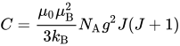
| the Avogadro constant | |
| µ0 | the permeability of free space. Note: in CGS units is taken to equal one.[29] |
| g | the Landé g-factor |
| J(J + 1) | the eigenvalue for eigenstate J2 for the stationary states within the incomplete atoms shells (electrons unpaired) |
| µB | the Bohr magneton |
| kB | the Boltzmann constant |
| total magnetism | is N number of magnetic moments per unit volume[clarification needed] |

The Curie–Weiss law is then derived from Curie's law to be:
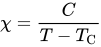
where:

λ is the Weiss molecular field constant.[28][30]
For full derivation see Curie–Weiss law.
Physics
[edit]Approaching Curie temperature from above
[edit]As the Curie–Weiss law is an approximation, a more accurate model is needed when the temperature, T, approaches the material's Curie temperature, TC.
Magnetic susceptibility occurs above the Curie temperature.
An accurate model of critical behaviour for magnetic susceptibility with critical exponent γ:

The critical exponent differs between materials and for the mean-field model is taken as γ = 1.[31]
As temperature is inversely proportional to magnetic susceptibility, when T approaches TC the denominator tends to zero and the magnetic susceptibility approaches infinity allowing magnetism to occur. This is a spontaneous magnetism which is a property of ferromagnetic and ferrimagnetic materials.[32][33]
Approaching Curie temperature from below
[edit]
Magnetism depends on temperature and spontaneous magnetism occurs below the Curie temperature. An accurate model of critical behaviour for spontaneous magnetism with critical exponent β:

The critical exponent differs between materials and for the mean-field model as taken as β = 1/2 where T ≪ TC.[31]
The spontaneous magnetism approaches zero as the temperature increases towards the materials Curie temperature.
Approaching absolute zero (0 kelvin)
[edit]The spontaneous magnetism, occurring in ferromagnetic, ferrimagnetic, and antiferromagnetic materials, approaches zero as the temperature increases towards the material's Curie temperature. Spontaneous magnetism is at its maximum as the temperature approaches 0 K.[35] That is, the magnetic moments are completely aligned and at their strongest magnitude of magnetism due to lack of thermal disturbance.
In paramagnetic materials thermal energy is sufficient to overcome the ordered alignments. As the temperature approaches 0 K, the entropy decreases to zero, that is, the disorder decreases and the material becomes ordered. This occurs without the presence of an applied magnetic field and obeys the third law of thermodynamics.[18]
Both Curie's law and the Curie–Weiss law fail as the temperature approaches 0 K. This is because they depend on the magnetic susceptibility, which only applies when the state is disordered.[36]
Gadolinium sulfate continues to satisfy Curie's law at 1 K. Between 0 and 1 K the law fails to hold and a sudden change in the intrinsic structure occurs at the Curie temperature.[37]
Ising model of phase transitions
[edit]The Ising model is mathematically based and can analyse the critical points of phase transitions in ferromagnetic order due to spins of electrons having magnitudes of ±1/2. The spins interact with their neighbouring dipole electrons in the structure and here the Ising model can predict their behaviour with each other.[38][39]
This model is important for solving and understanding the concepts of phase transitions and hence solving the Curie temperature. As a result, many different dependencies that affect the Curie temperature can be analysed.
For example, the surface and bulk properties depend on the alignment and magnitude of spins and the Ising model can determine the effects of magnetism in this system.
One should note, in 1D the Curie (critical) temperature for a magnetic order phase transition is found to be at zero temperature, i.e. the magnetic order takes over only at T = 0. In 2D, the critical temperature, e.g. a finite magnetization, can be calculated by solving the inequality:

Weiss domains and surface and bulk Curie temperatures
[edit]
Materials structures consist of intrinsic magnetic moments which are separated into domains called Weiss domains.[40] This can result in ferromagnetic materials having no spontaneous magnetism as domains could potentially balance each other out.[40] The position of particles can therefore have different orientations around the surface than the main part (bulk) of the material. This property directly affects the Curie temperature as there can be a bulk Curie temperature TB and a different surface Curie temperature TS for a material.[41]
This allows for the surface Curie temperature to be ferromagnetic above the bulk Curie temperature when the main state is disordered, i.e. ordered and disordered states occur simultaneously.[38]
The surface and bulk properties can be predicted by the Ising model and electron capture spectroscopy can be used to detect the electron spins and hence the magnetic moments on the surface of the material. An average total magnetism is taken from the bulk and surface temperatures to calculate the Curie temperature from the material, noting the bulk contributes more.[38][42]
The angular momentum of an electron is either +ħ/2 or −ħ/2 due to it having a spin of 1/2, which gives a specific size of magnetic moment to the electron; the Bohr magneton.[43] Electrons orbiting around the nucleus in a current loop create a magnetic field which depends on the Bohr magneton and magnetic quantum number.[43] Therefore, the magnetic moments are related between angular and orbital momentum and affect each other. Angular momentum contributes twice as much to magnetic moments than orbital.[44]
For terbium which is a rare-earth metal and has a high orbital angular momentum the magnetic moment is strong enough to affect the order above its bulk temperatures. It is said to have a high anisotropy on the surface, that is it is highly directed in one orientation. It remains ferromagnetic on its surface above its Curie temperature (219 K) while its bulk becomes antiferromagnetic and then at higher temperatures its surface remains antiferromagnetic above its bulk Néel Temperature (230 K) before becoming completely disordered and paramagnetic with increasing temperature. The anisotropy in the bulk is different from its surface anisotropy just above these phase changes as the magnetic moments will be ordered differently or ordered in paramagnetic materials.[41][45]
Changing a material's Curie temperature
[edit]Composite materials
[edit]Composite materials, that is, materials composed from other materials with different properties, can change the Curie temperature. For example, a composite which has silver in it can create spaces for oxygen molecules in bonding which decreases the Curie temperature[46] as the crystal lattice will not be as compact.
The alignment of magnetic moments in the composite material affects the Curie temperature. If the material's moments are parallel with each other, the Curie temperature will increase and if perpendicular the Curie temperature will decrease[46] as either more or less thermal energy will be needed to destroy the alignments.
Preparing composite materials through different temperatures can result in different final compositions which will have different Curie temperatures.[47] Doping a material can also affect its Curie temperature.[47]
The density of nanocomposite materials changes the Curie temperature. Nanocomposites are compact structures on a nano-scale. The structure is built up of high and low bulk Curie temperatures, however will only have one mean-field Curie temperature. A higher density of lower bulk temperatures results in a lower mean-field Curie temperature, and a higher density of higher bulk temperature significantly increases the mean-field Curie temperature. In more than one dimension the Curie temperature begins to increase as the magnetic moments will need more thermal energy to overcome the ordered structure.[42]
Particle size
[edit]The size of particles in a material's crystal lattice changes the Curie temperature. Due to the small size of particles (nanoparticles) the fluctuations of electron spins become more prominent, which results in the Curie temperature drastically decreasing when the size of particles decreases, as the fluctuations cause disorder. The size of a particle also affects the anisotropy causing alignment to become less stable and thus lead to disorder in magnetic moments.[38][48]
The extreme of this is superparamagnetism which only occurs in small ferromagnetic particles. In this phenomenon, fluctuations are very influential causing magnetic moments to change direction randomly and thus create disorder.
The Curie temperature of nanoparticles is also affected by the crystal lattice structure: body-centred cubic (bcc), face-centred cubic (fcc), and a hexagonal structure (hcp) all have different Curie temperatures due to magnetic moments reacting to their neighbouring electron spins. fcc and hcp have tighter structures and as a results have higher Curie temperatures than bcc as the magnetic moments have stronger effects when closer together.[38] This is known as the coordination number which is the number of nearest neighbouring particles in a structure. This indicates a lower coordination number at the surface of a material than the bulk which leads to the surface becoming less significant when the temperature is approaching the Curie temperature. In smaller systems the coordination number for the surface is more significant and the magnetic moments have a stronger effect on the system.[38]
Although fluctuations in particles can be minuscule, they are heavily dependent on the structure of crystal lattices as they react with their nearest neighbouring particles. Fluctuations are also affected by the exchange interaction[48] as parallel facing magnetic moments are favoured and therefore have less disturbance and disorder, therefore a tighter structure influences a stronger magnetism and therefore a higher Curie temperature.
Pressure
[edit]Pressure changes a material's Curie temperature. Increasing pressure on the crystal lattice decreases the volume of the system. Pressure directly affects the kinetic energy in particles as movement increases causing the vibrations to disrupt the order of magnetic moments. This is similar to temperature as it also increases the kinetic energy of particles and destroys the order of magnetic moments and magnetism.[49]
Pressure also affects the density of states (DOS).[49] Here the DOS decreases causing the number of electrons available to the system to decrease. This leads to the number of magnetic moments decreasing as they depend on electron spins. It would be expected because of this that the Curie temperature would decrease; however, it increases. This is the result of the exchange interaction. The exchange interaction favours the aligned parallel magnetic moments due to electrons being unable to occupy the same space in time[18] and as this is increased due to the volume decreasing the Curie temperature increases with pressure. The Curie temperature is made up of a combination of dependencies on kinetic energy and the DOS.[49]
The concentration of particles also affects the Curie temperature when pressure is being applied and can result in a decrease in Curie temperature when the concentration is above a certain percent.[49]
Orbital ordering
[edit]Orbital ordering changes the Curie temperature of a material. Orbital ordering can be controlled through applied strains.[50] This is a function that determines the wave of a single electron or paired electrons inside the material. Having control over the probability of where the electron will be allows the Curie temperature to be altered. For example, the delocalised electrons can be moved onto the same plane by applied strains within the crystal lattice.[50]
The Curie temperature is seen to increase greatly due to electrons being packed together in the same plane, they are forced to align due to the exchange interaction and thus increases the strength of the magnetic moments which prevents thermal disorder at lower temperatures.
Curie temperature in ferroelectric materials
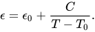
[edit]In analogy to ferromagnetic and paramagnetic materials, the term Curie temperature (TC) is also applied to the temperature at which a ferroelectric material transitions to being paraelectric. Hence, TC is the temperature where ferroelectric materials lose their spontaneous polarisation as a first or second order phase change occurs. In case of a second order transition, the Curie Weiss temperature T0 which defines the maximum of the dielectric constant is equal to the Curie temperature. However, the Curie temperature can be 10 K higher than T0 in case of a first order transition.[51]


| Below TC | Above TC[52] |
|---|---|
| Ferroelectric | ↔ Dielectric (paraelectric) |
| Antiferroelectric | ↔ Dielectric (paraelectric) |
| Ferrielectric | ↔ Dielectric (paraelectric) |
| Helielectric | ↔ Dielectric (paraelectric) |
Ferroelectric and dielectric
[edit]Materials are only ferroelectric below their corresponding transition temperature T0.[53] Ferroelectric materials are all pyroelectric and therefore have a spontaneous electric polarisation as the structures are unsymmetrical.
Ferroelectric materials' polarization is subject to hysteresis (Figure 4); that is they are dependent on their past state as well as their current state. As an electric field is applied the dipoles are forced to align and polarisation is created, when the electric field is removed polarisation remains. The hysteresis loop depends on temperature and as a result as the temperature is increased and reaches T0 the two curves become one curve as shown in the dielectric polarisation (Figure 5).[54]
Relative permittivity
[edit]A modified version of the Curie–Weiss law applies to the dielectric constant, also known as the relative permittivity:[51][55]
Applications
[edit]A heat-induced ferromagnetic-paramagnetic transition is used in magneto-optical storage media for erasing and writing of new data. Famous examples include the Sony Minidisc format as well as the now-obsolete CD-MO format. Curie point electro-magnets have been proposed and tested for actuation mechanisms in passive safety systems of fast breeder reactors, where control rods are dropped into the reactor core if the actuation mechanism heats up beyond the material's Curie point.[56] Other uses include temperature control in soldering irons[57] and stabilizing the magnetic field of tachometer generators against temperature variation.[58]
See also
[edit]- Ferroelectricity – Property of materials which both possess and are affected by electric fields
- Curie's law – Relation of magnetization to applied magnetic field and temperature
- Hopkinson effect – Feature of ferromagnetic or ferrimagnetic materials
Notes
[edit]- ^ Pierre Curie – Biography
- ^ Buschow 2001, p5021, table 1
- ^ Jullien & Guinier 1989, p. 155
- ^ Kittel 1986
- ^ Nigh, H. E.; Legvold, S.; Spedding, F. H. (1 November 1963). "Magnetization and Electrical Resistivity of Gadolinium Single Crystals". Physical Review. 132 (3): 1092–1097. Bibcode:1963PhRv..132.1092N. doi:10.1103/PhysRev.132.1092. ISSN 0031-899X.
- ^ a b Coey, J.M.D.; Mazaleyrat, Frédéric (2023). History of magnetism. Elsevier.
- ^ Hall & Hook 1994, p. 200
- ^ Jullien & Guinier 1989, pp. 136–38
- ^ a b Ibach & Lüth 2009
- ^ a b Levy 1968, pp. 236–39
- ^ Dekker 1958, pp. 217–20
- ^ Levy 1968
- ^ a b c Fan 1987, pp. 164–65
- ^ Dekker 1958, pp. 454–55
- ^ Mendelssohn 1977, p. 162
- ^ Levy 1968, pp. 198–202
- ^ a b c Cusack 1958, p. 269
- ^ a b c d Hall & Hook 1994, pp. 220–21
- ^ Palmer 2007
- ^ Hall & Hook 1994, p. 220
- ^ a b c d Jullien & Guinier 1989, pp. 158–59
- ^ Spaldin, Nicola A. (2006). Magnetic materials: fundamentals and device applications (Repr. ed.). Cambridge: Cambridge Univ. Press. pp. 89–106. ISBN 978-0-521-01658-2.
- ^ a b Jullien & Guinier 1989, pp. 156–57
- ^ Kittel, Charles (2005). Introduction to Solid State Physics (8th ed.). New York: John Wiley & Sons. ISBN 978-0-471-41526-8.
- ^ Ichida, Toshio (1973). "Mössbauer Study of the Thermal Decomposition Products of K2FeO4". Bulletin of the Chemical Society of Japan. 46 (1): 79–82. doi:10.1246/bcsj.46.79.
- ^ Jullien & Guinier 1989, pp. 153
- ^ Hall & Hook 1994, pp. 205–06
- ^ a b Levy 1968, pp. 201–02
- ^ Kittel 1996, p. 444
- ^ Myers 1997, pp. 334–345
- ^ a b Hall & Hook 1994, pp. 227–28
- ^ Kittel 1986, pp. 424–26
- ^ Spaldin 2010, pp. 52–54
- ^ Adapted from T Chatterji, M Zamponi, J Wuttke: Hyperfine interaction in cobalt by high-resolution neutron spectroscopy. J Phys: Condens Matter 31, 025801 (2019), Fig 4.
- ^ Hall & Hook 1994, p. 225
- ^ Mendelssohn 1977, pp. 180–81
- ^ Mendelssohn 1977, p. 167
- ^ a b c d e f Bertoldi, Bringa & Miranda 2012
- ^ Brout 1965, pp. 6–7
- ^ a b Jullien & Guinier 1989, p. 161
- ^ a b Rau, Jin & Robert 1988
- ^ a b Skomski & Sellmyer 2000
- ^ a b Jullien & Guinier 1989, p. 138
- ^ Hall & Hook 1994
- ^ Jackson, M. (2000). "Magnetism of Rare Earth" (PDF). The IRM Quarterly. 10 (3): 1. Archived from the original (PDF) on 12 July 2017. Retrieved 21 January 2020.
- ^ a b Hwang et al. 1998
- ^ a b Paulsen et al. 2003
- ^ a b López Domínguez et al. 2013
- ^ a b c d Bose et al. 2011
- ^ a b Sadoc et al. 2010
- ^ a b Webster 1999
- ^ Kovetz 1990, p. 116
- ^ Myers 1997, pp. 404–05
- ^ Pascoe 1973, pp. 190–91
- ^ Webster 1999, pp. 6.55–6.56
- ^ Takamatsu (2007). "Demonstration of Control Rod Holding Stability of the Self Actuated Shutdown System in Joyo for Enhancement of Fast Reactor Inherent Safety". Journal of Nuclear Science and Technology. 44 (3): 511–517. Bibcode:2007JNST...44..511T. doi:10.1080/18811248.2007.9711316.
- ^ TMT-9000S
- ^ Pallàs-Areny & Webster 2001, pp. 262–63
References
[edit]- Buschow, K. H. J. (2001). Encyclopedia of Materials: Science and Technology. Elsevier. ISBN 0-08-043152-6.
- Kittel, Charles (1986). Introduction to Solid State Physics (6th ed.). John Wiley & Sons. ISBN 0-471-87474-4.
- Pallàs-Areny, Ramon; Webster, John G. (2001). Sensors and Signal Conditioning (2nd ed.). John Wiley & Sons. ISBN 978-0-471-33232-9.
- Spaldin, Nicola A. (2010). Magnetic Materials: Fundamentals and Applications (2nd ed.). Cambridge: Cambridge University Press. ISBN 978-0-521-88669-7.
- Ibach, Harald; Lüth, Hans (2009). Solid-State Physics: An Introduction to Principles of Materials Science (4th ed.). Berlin: Springer. ISBN 978-3-540-93803-3.
- Levy, Robert A. (1968). Principles of Solid State Physics. Academic Press. ISBN 978-0-12-445750-8.
- Fan, H. Y. (1987). Elements of Solid State Physics. Wiley-Interscience. ISBN 978-0-471-85987-1.
- Dekker, Adrianus J. (1958). Solid State Physics. Macmillan. ISBN 978-0-333-10623-5.
{{cite book}}: ISBN / Date incompatibility (help) - Cusack, N. (1958). The Electrical and Magnetic Properties of Solids. Longmans, Green.
- Hall, J. R.; Hook, H. E. (1994). Solid State Physics (2nd ed.). Chichester: Wiley. ISBN 0-471-92805-4.
- Jullien, André; Guinier, Rémi (1989). The Solid State from Superconductors to Superalloys. Oxford: Oxford Univ. Press. ISBN 0-19-855554-7.
- Mendelssohn, K. (1977). The Quest for Absolute Zero: The Meaning of Low Temperature Physics. with S.I. units. (2nd ed.). London: Taylor and Francis. ISBN 0-85066-119-6.
- Myers, H. P. (1997). Introductory Solid State Physics (2nd ed.). London: Taylor & Francis. ISBN 0-7484-0660-3.
- Kittel, Charles (1996). Introduction to Solid State Physics (7th ed.). New York [u.a.]: Wiley. ISBN 0-471-11181-3.
- Palmer, John (2007). Planar Ising correlations (Online ed.). Boston: Birkhäuser. ISBN 978-0-8176-4620-2.
- Bertoldi, Dalía S.; Bringa, Eduardo M.; Miranda, E. N. (May 2012). "Analytical solution of the mean field Ising model for finite systems". Journal of Physics: Condensed Matter. 24 (22) 226004. Bibcode:2012JPCM...24v6004B. doi:10.1088/0953-8984/24/22/226004. hdl:11336/16945. PMID 22555147. S2CID 34323416. Retrieved 12 February 2013.
- Brout, Robert (1965). Phase Transitions. New York, Amsterdam: W. A. Benjamin, Inc.
- Rau, C.; Jin, C.; Robert, M. (1988). "Ferromagnetic order at Tb surfaces above the bulk Curie temperature". Journal of Applied Physics. 63 (8): 3667. Bibcode:1988JAP....63.3667R. doi:10.1063/1.340679.
- Skomski, R.; Sellmyer, D. J. (2000). "Curie temperature of multiphase nanostructures". Journal of Applied Physics. 87 (9): 4756. Bibcode:2000JAP....87.4756S. doi:10.1063/1.373149. S2CID 288790.
- López Domínguez, Victor; Hernàndez, Joan Manel; Tejada, Javier; Ziolo, Ronald F. (14 November 2012). "Colossal Reduction in Curie Temperature Due to Finite-Size Effects in CoFe
2O
4 Nanoparticles". Chemistry of Materials. 25 (1): 6–11. doi:10.1021/cm301927z. - Bose, S. K.; Kudrnovský, J.; Drchal, V.; Turek, I. (18 November 2011). "Pressure dependence of Curie temperature and resistivity in complex Heusler alloys". Physical Review B. 84 (17) 174422. arXiv:1010.3025. Bibcode:2011PhRvB..84q4422B. doi:10.1103/PhysRevB.84.174422. S2CID 118595011.
- Webster, John G., ed. (1999). The Measurement, Instrumentation, and Sensors Handbook (Online ed.). Boca Raton, FL: CRC Press published in cooperation with IEEE Press. ISBN 0-8493-8347-1.
- Whatmore, R. W. (1991). Electronic Materials: From Silicon to Organics (2nd ed.). New York, NY: Springer. ISBN 978-1-4613-6703-1.
- Kovetz, Attay (1990). The Principles of Electromagnetic Theory (1st ed.). Cambridge, UK: Cambridge University Press. ISBN 0-521-39997-1.
- Hummel, Rolf E. (2001). Electronic Properties of Materials (3rd ed.). New York [u.a.]: Springer. ISBN 0-387-95144-X.
- Pascoe, K. J. (1973). Properties of Materials for Electrical Engineers. New York, N.Y.: J. Wiley and Sons. ISBN 0-471-66911-3.
- Paulsen, J. A.; Lo, C. C. H.; Snyder, J. E.; Ring, A. P.; Jones, L. L.; Jiles, D. C. (23 September 2003). "Study of the Curie temperature of cobalt ferrite based composites for stress sensor applications". IEEE Transactions on Magnetics. 39 (5): 3316–18. Bibcode:2003ITM....39.3316P. doi:10.1109/TMAG.2003.816761. ISSN 0018-9464. S2CID 45734431.
- Hwang, Hae Jin; Nagai, Toru; Ohji, Tatsuki; Sando, Mutsuo; Toriyama, Motohiro; Niihara, Koichi (March 1998). "Curie temperature Anomaly in Lead Zirconate Titanate/Silver Composites". Journal of the American Ceramic Society. 81 (3): 709–12. doi:10.1111/j.1151-2916.1998.tb02394.x.
- Sadoc, Aymeric; Mercey, Bernard; Simon, Charles; Grebille, Dominique; Prellier, Wilfrid; Lepetit, Marie-Bernadette (2010). "Large Increase of the Curie temperature by Orbital Ordering Control". Physical Review Letters. 104 (4) 046804. arXiv:0910.3393. Bibcode:2010PhRvL.104d6804S. doi:10.1103/PhysRevLett.104.046804. PMID 20366729. S2CID 35041713.
- Kochmański, Martin; Paszkiewicz, Tadeusz; Wolski, Sławomir (2013). "Curie–Weiss magnet: a simple model of phase transition". European Journal of Physics. 34 (6): 1555–73. arXiv:1301.2141. Bibcode:2013EJPh...34.1555K. doi:10.1088/0143-0807/34/6/1555. S2CID 118331770.
- "Pierre Curie – Biography". Nobelprize.org. Nobel Media AB. 2014. Retrieved 14 March 2013.
- "TMT-9000S Soldering and Rework Station". thermaltronics.com. Retrieved 13 January 2016.
External links
[edit]
Curie temperature
View on GrokipediaBasic Concepts
Definition
The Curie temperature, denoted as $ T_c $, is the critical temperature at which ferromagnetic or ferrimagnetic materials undergo a phase transition, losing their long-range magnetic order and transitioning to a paramagnetic state.[6] In this transition, the spontaneous magnetization $ M_s $ vanishes precisely at $ T_c $; below $ T_c $, atomic magnetic moments align spontaneously due to dominant exchange interactions, forming ordered domains, whereas above $ T_c $, thermal energy disrupts this alignment, randomizing the spin orientations and eliminating net magnetization in the absence of an external field.[7][4] In the ideal case, the spontaneous magnetization satisfies $ M_s = 0 $ for $ T > T_c $.[7] The Curie temperature is expressed in kelvin (K) and serves as a key parameter in the study of second-order phase transitions, where the behavior of physical quantities near $ T_c $ is characterized by universal critical exponents, such as the exponent $ \beta $ describing how $ M_s $ approaches zero as $ T $ nears $ T_c $ from below.[8] Above $ T_c $, the inverse magnetic susceptibility $ \chi^{-1} $ follows the Curie-Weiss law, providing a related measure of paramagnetic behavior.[9] Experimentally, $ T_c $ is determined through techniques such as measuring the temperature dependence of magnetization using a vibrating sample magnetometer (VSM), where $ T_c $ is identified as the point where $ M_s $ extrapolates to zero, or via magnetic susceptibility measurements, in which a peak or inflection in $ \chi(T) $ signals the transition.[8][9] Hysteresis loop analysis also reveals $ T_c $ as the temperature where the coercive field and remanence diminish to zero, marking the loss of ferromagnetic hysteresis.[10]Significance in Phase Transitions
The Curie temperature marks the boundary between ferromagnetic and paramagnetic phases in magnetic materials, representing a classic example of a second-order phase transition where the order parameter—spontaneous magnetization—varies continuously to zero as the temperature approaches $ T_c $ from below, without abrupt structural changes.[8][11] Unlike first-order transitions, such as melting, there is no latent heat associated with the Curie point, allowing the system to evolve smoothly through the critical region.[12][13] This transition exemplifies critical phenomena, where physical properties near $ T_c $ follow universal scaling laws independent of microscopic details, governed by renormalization group theory that classifies systems into universality classes based on dimensionality, symmetry, and interaction range.[14] For three-dimensional ferromagnets with short-range interactions, the Curie transition belongs to the 3D Ising universality class, characterized by critical exponents such as for the order parameter and for susceptibility, reflecting shared behavior with other Ising-like systems.[15][16] These scaling relations enable predictive modeling of fluctuations and correlations that diverge at $ T_c $, with the correlation length growing as where .[14] At the Curie temperature, key thermodynamic properties exhibit singular behavior: the magnetic susceptibility diverges as , signaling enhanced responsiveness to external fields, while the specific heat shows a discontinuity or sharp anomaly, reflecting the onset of long-range order without volume changes.[17][18] In the modern context, investigations into low-dimensional systems, such as two-dimensional ferromagnets like FeGeTe, have revealed quantum critical points near $ T_c $ where thermal fluctuations interplay with quantum effects, leading to enhanced critical fluctuations and potential non-Fermi liquid behaviors, as evidenced by recent noise spectroscopy and theoretical studies up to 2025.[19][20]Historical Development
Pierre Curie's Discovery
In 1895, Pierre Curie, a physicist at the University of Paris (Sorbonne), conducted extensive experimental research on the magnetic properties of various materials as a function of temperature, which formed the basis of his doctoral thesis titled Propriétés magnétiques des corps à diverses températures.[21] This work, defended on March 6, 1895, before the Faculty of Sciences, marked a pivotal moment in the study of magnetism, as Curie systematically investigated how temperature influences magnetization in both paramagnetic and ferromagnetic substances.[21] His experiments were motivated by earlier observations on paramagnetism but extended to explore the behavior of strongly magnetic materials like iron, nickel, and cobalt under varying thermal conditions.[22] Curie's experimental setup involved a highly sensitive torsion balance, which he designed and refined to measure magnetic susceptibility with a resolution of 0.01 mg, combined with electromagnets to apply controlled magnetic fields and heating apparatus to vary sample temperatures precisely.[23] By suspending small samples of materials such as iron in the balance and observing deflections in the presence of a magnetic field while gradually increasing the temperature, Curie documented the loss of spontaneous magnetization in ferromagnetic samples at a specific critical threshold.[21] For instance, in iron, this transition occurred around 770°C, above which the material no longer exhibited ferromagnetic properties and instead behaved as a paramagnet, with no residual magnetism in the absence of an external field.[1] This phenomenon, initially referred to as the "Curie point," represented the temperature at which the material's magnetic domains disordered under thermal agitation.[21] A key observation from these experiments was that, above the Curie point, the magnetic susceptibility of formerly ferromagnetic materials followed an inverse relationship with absolute temperature, χ ∝ 1/T, mirroring the behavior Curie had already established for paramagnets in the same thesis—now known as Curie's law.[21] This empirical finding demonstrated that the paramagnetic phase of ferromagnets adheres to the same temperature dependence as inherent paramagnets, highlighting a continuity in magnetic response across material types once the critical temperature is surpassed.[22] These discoveries predated the quantum mechanical understanding of magnetism by decades, relying solely on classical phenomenological observations.[21]Theoretical Contributions
Following Pierre Curie's experimental discovery of the temperature above which ferromagnets lose their spontaneous magnetization, theoretical efforts sought to explain this Curie temperature through microscopic mechanisms. In 1907, Pierre-Ernest Weiss introduced the molecular field theory, proposing that ferromagnetism arises from an internal "molecular field" acting on atomic magnetic moments, analogous to an external field but proportional to the average magnetization. This mean-field approach successfully predicted a finite Curie temperature where thermal agitation overcomes the aligning effect of this internal field, marking a foundational step in understanding cooperative magnetic ordering. Building on Weiss's classical framework, Werner Heisenberg developed a quantum mechanical description in 1928, attributing ferromagnetism to exchange interactions between electron spins. In the Heisenberg model, the Curie temperature emerges from these quantum exchange energies, with a simplified relation given by $ T_c \approx \frac{z J}{k_B} $, where $ z $ is the number of nearest neighbors, $ J $ is the exchange constant $ J_{ij} $, and $ k_B $ is Boltzmann's constant. This quantum perspective shifted explanations from phenomenological fields to fundamental electron interactions, resolving inconsistencies in classical theories.[24] The mean-field approximation was further refined within the Heisenberg model, yielding the Curie temperature as $ T_c = \frac{2 z J S (S+1)}{3 k_B} $ for spins of magnitude $ S $, providing a quantitative link between microscopic exchange and the transition temperature. Key advancements came from Felix Bloch, who in 1930 incorporated band structure effects into quantum ferromagnetism, explaining low-temperature magnetization curves, and Lev Landau, whose 1937 phenomenological theory of second-order phase transitions described the Curie point through symmetry breaking and free-energy expansions near criticality.[25] Subsequent developments transitioned from these early classical and semi-classical models to fully quantum treatments, with post-1950s renormalization group methods revolutionizing precise calculations of critical behavior around the Curie temperature by accounting for fluctuations beyond mean-field limits. Pioneered by Kenneth Wilson, this approach clarified universal scaling laws and critical exponents influencing $ T_c $ estimates in complex systems.[26][27]Materials and Examples
Ferromagnetic and Ferrimagnetic Materials
Ferromagnetic materials, such as iron, nickel, and cobalt, display spontaneous magnetization and high magnetic permeability below their Curie temperature due to aligned magnetic moments in their lattice structures. Iron, with a body-centered cubic (bcc) structure, has a Curie temperature of 1043 K, while nickel in a face-centered cubic (fcc) structure exhibits a Curie temperature of 627 K, and cobalt in a hexagonal close-packed (hcp) structure reaches 1388 K. These properties make them essential for applications requiring strong, permanent magnetism at ambient conditions. Ferrimagnetic materials achieve net magnetization through antiparallel alignment of magnetic sublattices with unequal moments, as seen in oxides like magnetite (Fe₃O₄), which has an inverse spinel structure and a Curie temperature of 858 K. Ferrites, including NiZn variants such as Ni₀.₅Zn₀.₅Fe₂O₄ with a spinel structure, typically have Curie temperatures ranging from 300 K to 500 K, enabling their use in high-frequency devices. At the Curie temperature, both ferromagnetic and ferrimagnetic materials lose long-range net magnetization and become paramagnetic, though short-range magnetic order persists immediately above this point. In industrial contexts, pure ferromagnetic elements like iron and nickel serve as foundational materials for electromagnets and transformers, whereas alloys such as permalloy (Ni₈₀Fe₂₀, fcc structure, Curie temperature ≈800 K) offer enhanced soft magnetic properties with lower coercivity for shielding and sensor applications. The following table summarizes Curie temperatures for selected ferromagnetic and ferrimagnetic materials, including notes on their crystal structures:| Material | Curie Temperature (K) | Crystal Structure Notes |
|---|---|---|
| Iron (Fe) | 1043 | Body-centered cubic (bcc) |
| Nickel (Ni) | 627 | Face-centered cubic (fcc) |
| Cobalt (Co) | 1388 | Hexagonal close-packed (hcp) |
| Magnetite (Fe₃O₄) | 858 | Inverse spinel |
| Nickel ferrite (NiFe₂O₄) | 858 | Spinel |
| Permalloy (Ni₈₀Fe₂₀) | ≈800 | Face-centered cubic (fcc) |
| NiZn ferrite (e.g., Ni₀.₅Zn₀.₅Fe₂O₄) | ≈450 | Spinel |
Paramagnetic and Antiferromagnetic Behaviors
In ferromagnetic materials, the region above the Curie temperature is characterized by paramagnetic behavior, where thermal agitation disrupts the aligned magnetic moments, eliminating spontaneous magnetization and leaving the material responsive only to external fields.[28] In this state, the magnetic susceptibility follows the Curie law, expressed as , where is the material-specific Curie constant and is the absolute temperature; this relation arises from the random orientation of independent magnetic moments.[29] Intrinsic paramagnetic materials, lacking any underlying ordered phase, do not exhibit a Curie temperature, as their susceptibility adheres to the same Curie law across all temperatures without a phase transition.[29] Antiferromagnetic materials feature a structural analog to the Curie temperature known as the Néel temperature , below which neighboring spins align in antiparallel configurations through dominant antiferromagnetic exchange interactions, yielding no net magnetization despite the ordered state.[30] At , this antiparallel order breaks down, transitioning the material to a paramagnetic phase where spins are thermally disordered.[30] Unlike ferromagnets, the magnetic susceptibility in antiferromagnets typically reaches a maximum at due to enhanced short-range correlations near the transition, rather than following a simple monotonic decrease.[30] Representative examples include manganese(II) oxide (MnO), with K, and elemental chromium, with K for strain-free single crystals.[31][32] In certain compounds with competing ferromagnetic and antiferromagnetic exchange interactions, the Curie temperature and Néel temperature can coexist or sequence differently, such as when ferromagnetic coupling dominates overall or in cases favoring antiferromagnetic sublattices, influencing the resulting magnetic ground state.[33][34] This competition highlights distinctions from purely ferromagnetic systems, where net magnetization persists below , as antiferromagnetic order inherently cancels macroscopic moments even in the low-temperature phase.[30]Theoretical Foundations
Curie-Weiss Law
The Curie-Weiss law governs the temperature dependence of the magnetic susceptibility in ferromagnetic materials above the Curie temperature , expressed asMean-Field Approximations Near Tc
In mean-field theory, the thermodynamic behavior near the Curie temperature $ T_c $ is captured through a phenomenological expansion of the free energy density in terms of the magnetization $ m $, serving as the order parameter for the ferromagnetic phase transition. The standard form, known as the Landau free energy, isAdvanced Physics
Ising Model and Critical Phenomena
The Ising model provides a foundational lattice-based framework for understanding magnetic phase transitions, particularly the emergence of spontaneous magnetization at the Curie temperature . In this model, spins are placed at lattice sites, interacting via nearest-neighbor couplings, with the system's energy described by the HamiltonianDomain Theory and Low-Temperature Limits
In ferromagnetic materials below the Curie temperature , the spontaneous magnetization leads to the formation of magnetic domains, as proposed by Pierre Weiss in 1907 to explain the observed low magnetization in the absence of an external field.[41] These domains are extended regions where the atomic magnetic moments are aligned parallel within each domain but oriented in different directions across domains, thereby minimizing the magnetostatic (demagnetization) energy associated with free magnetic poles on the material's surface. The boundaries between adjacent domains, known as domain walls or Bloch walls, are narrow transition zones—typically tens to hundreds of nanometers thick—where the magnetization rotates gradually from one domain direction to another, balancing exchange energy and magnetocrystalline anisotropy to further reduce the total energy.[41] At low temperatures approaching absolute zero ( K), the magnetization reaches its saturation value , with all spins fully aligned due to dominant exchange interactions. However, thermal excitations give rise to spin waves (magnons), which cause a slight reduction in the net magnetization. This temperature dependence is described by Bloch's law, derived from quantum mechanical considerations of spin-wave theory:Modifying the Curie Temperature
Effects of Pressure and Composition
The application of hydrostatic pressure to ferromagnetic materials generally leads to a decrease in the Curie temperature (Tc), with the pressure derivative dTc/dP being negative for most 3d transition metal ferromagnets due to the compression-induced weakening of magnetic exchange interactions. This effect arises from the reduction in atomic volume, which alters the overlap of electron wavefunctions and consequently impacts the strength of direct or indirect exchange coupling between magnetic moments. For instance, in body-centered cubic (bcc) iron, experimental and theoretical studies indicate a near-zero dTc/dP (experimentally ≈ 0 K/GPa), reflecting the delicate balance in its itinerant electron magnetism.[42][43] In contrast, certain rare-earth based compounds exhibit positive dTc/dP, where pressure enhances exchange pathways; for example, in Gd5(SixGe1-x)4 alloys near x=0.5, dTc/dP reaches +1.2 K/kbar (+12 K/GPa), attributed to pressure-stabilized ferromagnetic ordering in the magnetocaloric phase.[44] The sign and magnitude of dTc/dP depend on the material's electronic structure and the nature of its magnetism. In localized-spin systems like gadolinium metal, pressure typically depresses Tc at a rate of about -1.6 K/kbar (-16 K/GPa) up to moderate pressures, as the compressed lattice reduces the indirect RKKY exchange via conduction electrons.[45] However, in some van der Waals ferromagnets such as VI3, pressure dramatically increases Tc from ~50 K at ambient conditions to over 250 K at 2.5 GPa, with dTc/dP exceeding +80 K/GPa in the low-pressure regime, driven by enhanced interlayer coupling.[46]| Material | dTc/dP (K/GPa) | Notes |
|---|---|---|
| bcc Fe | ≈ 0 | Itinerant ferromagnet; essential independence from ab initio and experiment.[42] |
| Ni | -3.6 | fcc structure; typical for 3d metals.[47] |
| Gd | -16 | Localized moments; linear decrease up to 2 GPa.[45] |
| Gd5Si2Ge2 | +12 | Giant magnetocaloric; positive shift stabilizes ferromagnetism.[44] |
| VI3 | +80 (initial) | 2D ferromagnet; huge enhancement via interlayer exchange.[46] |