Community hub
Hypergeometric distribution
View on Wikipedia
| Hypergeometric | |||
|---|---|---|---|
|
Probability mass function  | |||
|
Cumulative distribution function  | |||
| Parameters | |||
| Support | |||
| PMF | |||
| CDF | where is the generalized hypergeometric function | ||
| Mean | |||
| Mode | |||
| Variance | |||
| Skewness | |||
| Excess kurtosis |
| ||
| MGF | |||
| CF | |||


![{\displaystyle 1-{{{n \choose {k+1}}{{N-n} \choose {K-k-1}}} \over {N \choose K}}\,_{3}F_{2}\!\!\left[{\begin{array}{c}1,\ k+1-K,\ k+1-n\\k+2,\ N+k+2-K-n\end{array}};1\right],}](https://wikimedia.org/api/rest_v1/media/math/render/svg/556153b7446bc4321c995b2d8f9cc2957a0df452)


![{\displaystyle {\frac {(N-2K)(N-1)^{\frac {1}{2}}(N-2n)}{[nK(N-K)(N-n)]^{\frac {1}{2}}(N-2)}}}](https://wikimedia.org/api/rest_v1/media/math/render/svg/f9ec1b0c28225251fa3fd794e30bffc3eb34315e)


![{\displaystyle {}+6nK(N-K)(N-n)(5N-6){\big ]}}](https://wikimedia.org/api/rest_v1/media/math/render/svg/873d966636267a7d676f2d26681eb7bcf1a2259b)


In probability theory and statistics, the hypergeometric distribution is a discrete probability distribution that describes the probability of successes (random draws for which the object drawn has a specified feature) in draws, without replacement, from a finite population of size that contains exactly objects with that feature, where in each draw is either a success or a failure. In contrast, the binomial distribution describes the probability of successes in draws with replacement.


Definitions
[edit]Probability mass function
[edit]The following conditions characterize the hypergeometric distribution:
- The result of each draw (the elements of the population being sampled) can be classified into one of two mutually exclusive categories (e.g. Pass/Fail or Employed/Unemployed).
- The probability of a success changes on each draw, as each draw decreases the population (sampling without replacement from a finite population).
A random variable follows the hypergeometric distribution if its probability mass function (pmf) is given by[1]


where
- is the population size,
- is the number of success states in the population,
- is the number of draws (i.e. quantity drawn in each trial),
- is the number of observed successes,
- is a binomial coefficient.

The pmf is positive when .

A random variable distributed hypergeometrically with parameters , and is written and has probability mass function above.


Combinatorial identities
[edit]As required, we have

which essentially follows from Vandermonde's identity from combinatorics.
Also note that

This identity can be shown by expressing the binomial coefficients in terms of factorials and rearranging the latter. Additionally, it follows from the symmetry of the problem, described in two different but interchangeable ways.
For example, consider two rounds of drawing without replacement. In the first round, out of neutral marbles are drawn from an urn without replacement and coloured green. Then the colored marbles are put back. In the second round, marbles are drawn without replacement and colored red. Then, the number of marbles with both colors on them (that is, the number of marbles that have been drawn twice) has the hypergeometric distribution. The symmetry in and stems from the fact that the two rounds are independent, and one could have started by drawing balls and colouring them red first.
Note that we are interested in the probability of successes in draws without replacement, since the probability of success on each trial is not the same, as the size of the remaining population changes as we remove each marble. Keep in mind not to confuse with the binomial distribution, which describes the probability of successes in draws with replacement.
Properties
[edit]Working example
[edit]The classical application of the hypergeometric distribution is sampling without replacement. Think of an urn with two colors of marbles, red and green. Define drawing a green marble as a success and drawing a red marble as a failure. Let N describe the number of all marbles in the urn (see contingency table below) and K describe the number of green marbles, then N − K corresponds to the number of red marbles. Now, standing next to the urn, you close your eyes and draw n marbles without replacement. Define X as a random variable whose outcome is k, the number of green marbles drawn in the experiment. This situation is illustrated by the following contingency table:
| drawn | not drawn | total | |
|---|---|---|---|
| green marbles | k | K − k | K |
| red marbles | n − k | N + k − n − K | N − K |
| total | n | N − n | N |
Indeed, we are interested in calculating the probability of drawing k green marbles in n draws, given that there are K green marbles out of a total of N marbles. For this example, assume that there are 5 green and 45 red marbles in the urn. Standing next to the urn, you close your eyes and draw 10 marbles without replacement. What is the probability that exactly 4 of the 10 are green?
This problem is summarized by the following contingency table:
| drawn | not drawn | total | |
|---|---|---|---|
| green marbles | k = 4 | K − k = 1 | K = 5 |
| red marbles | n − k = 6 | N + k − n − K = 39 | N − K = 45 |
| total | n = 10 | N − n = 40 | N = 50 |
To find the probability of drawing k green marbles in exactly n draws out of N total draws, we identify X as a hyper-geometric random variable to use the formula

To intuitively explain the given formula, consider the two symmetric problems represented by the identity

- left-hand side - drawing a total of only n marbles out of the urn. We want to find the probability of the outcome of drawing k green marbles out of K total green marbles, and drawing n-k red marbles out of N-K red marbles, in these n rounds.
- right hand side - alternatively, drawing all N marbles out of the urn. We want to find the probability of the outcome of drawing k green marbles in n draws out of the total N draws, and K-k green marbles in the rest N-n draws.
Back to the calculations, we use the formula above to calculate the probability of drawing exactly k green marbles

Intuitively we would expect it to be even more unlikely that all 5 green marbles will be among the 10 drawn.

As expected, the probability of drawing 5 green marbles is roughly 35 times less likely than that of drawing 4.
Symmetries
[edit]Swapping the roles of green and red marbles:

Swapping the roles of drawn and not drawn marbles:

Swapping the roles of green and drawn marbles:

These symmetries generate the dihedral group .

Order of draws
[edit]The probability of drawing any set of green and red marbles (the hypergeometric distribution) depends only on the numbers of green and red marbles, not on the order in which they appear; i.e., it is an exchangeable distribution. As a result, the probability of drawing a green marble in the draw is[2]


This is an ex ante probability—that is, it is based on not knowing the results of the previous draws.
Tail bounds
[edit]Let and . Then for we can derive the following bounds:[3]


![{\displaystyle {\begin{aligned}\Pr[X\leq (p-t)n]&\leq e^{-n{\text{D}}(p-t\parallel p)}\leq e^{-2t^{2}n}\\\Pr[X\geq (p+t)n]&\leq e^{-n{\text{D}}(p+t\parallel p)}\leq e^{-2t^{2}n}\\\end{aligned}}\!}](https://wikimedia.org/api/rest_v1/media/math/render/svg/c1592b043d16fd6179f3a95d97a3c38806d82cea)
where

is the Kullback–Leibler divergence and it is used that .[4]

Note: In order to derive the previous bounds, one has to start by observing that where are dependent random variables with a specific distribution . Because most of the theorems about bounds in sum of random variables are concerned with independent sequences of them, one has to first create a sequence of independent random variables with the same distribution and apply the theorems on . Then, it is proved from Hoeffding [3] that the results and bounds obtained via this process hold for as well.


If n is larger than N/2, it can be useful to apply symmetry to "invert" the bounds, which give you the following: [4] [5]
![{\displaystyle {\begin{aligned}\Pr[X\leq (p-t)n]&\leq e^{-(N-n){\text{D}}(p+{\tfrac {tn}{N-n}}||p)}\leq e^{-2t^{2}n{\tfrac {n}{N-n}}}\\\\\Pr[X\geq (p+t)n]&\leq e^{-(N-n){\text{D}}(p-{\tfrac {tn}{N-n}}||p)}\leq e^{-2t^{2}n{\tfrac {n}{N-n}}}\\\end{aligned}}\!}](https://wikimedia.org/api/rest_v1/media/math/render/svg/a0fd3b1453cac4e9cd1a15a032c154bbb93b7ec4)
Statistical Inference
[edit]Hypergeometric test
[edit]The hypergeometric test uses the hypergeometric distribution to measure the statistical significance of having drawn a sample consisting of a specific number of successes (out of total draws) from a population of size containing successes. In a test for over-representation of successes in the sample, the hypergeometric p-value is calculated as the probability of randomly drawing or more successes from the population in total draws. In a test for under-representation, the p-value is the probability of randomly drawing or fewer successes.

The test based on the hypergeometric distribution (hypergeometric test) is identical to the corresponding one-tailed version of Fisher's exact test.[6] Reciprocally, the p-value of a two-sided Fisher's exact test can be calculated as the sum of two appropriate hypergeometric tests (for more information see[7]).
The test is often used to identify which sub-populations are over- or under-represented in a sample. This test has a wide range of applications. For example, a marketing group could use the test to understand their customer base by testing a set of known customers for over-representation of various demographic subgroups (e.g., women, people under 30).
Related distributions
[edit]Let and .
- If then has a Bernoulli distribution with parameter .
- Let have a binomial distribution with parameters and ; this models the number of successes in the analogous sampling problem with replacement. If and are large compared to , and is not close to 0 or 1, then and have similar distributions, i.e., .
- If is large, and are large compared to , and is not close to 0 or 1, then


where is the standard normal distribution function

- If the probabilities of drawing a green or red marble are not equal (e.g. because green marbles are bigger/easier to grasp than red marbles) then has a noncentral hypergeometric distribution
- The beta-binomial distribution is a conjugate prior for the hypergeometric distribution.
The following table describes four distributions related to the number of successes in a sequence of draws:
| With replacements | No replacements | |
|---|---|---|
| Given number of draws | binomial distribution | hypergeometric distribution |
| Given number of failures | negative binomial distribution | negative hypergeometric distribution |
Multivariate hypergeometric distribution
[edit]| Multivariate hypergeometric distribution | |||
|---|---|---|---|
| Parameters |
| ||
| Support | |||
| PMF | |||
| Mean | |||
| Variance |
| ||


The model of an urn with green and red marbles can be extended to the case where there are more than two colors of marbles. If there are Ki marbles of color i in the urn and you take n marbles at random without replacement, then the number of marbles of each color in the sample (k1, k2,..., kc) has the multivariate hypergeometric distribution:

This has the same relationship to the multinomial distribution that the hypergeometric distribution has to the binomial distribution—the multinomial distribution is the "with-replacement" distribution and the multivariate hypergeometric is the "without-replacement" distribution.
The properties of this distribution are given in the adjacent table,[8] where c is the number of different colors and is the total number of marbles in the urn.
Example
[edit]Suppose there are 5 black, 10 white, and 15 red marbles in an urn. If six marbles are chosen without replacement, the probability that exactly two of each color are chosen is

Occurrence and applications
[edit]Application to auditing elections
[edit]
Election audits typically test a sample of machine-counted precincts to see if recounts by hand or machine match the original counts. Mismatches result in either a report or a larger recount. The sampling rates are usually defined by law, not statistical design, so for a legally defined sample size n, what is the probability of missing a problem which is present in K precincts, such as a hack or bug? This is the probability that k = 0 . Bugs are often obscure, and a hacker can minimize detection by affecting only a few precincts, which will still affect close elections, so a plausible scenario is for K to be on the order of 5% of N. Audits typically cover 1% to 10% of precincts (often 3%),[9][10][11] so they have a high chance of missing a problem. For example, if a problem is present in 5 of 100 precincts, a 3% sample has 86% probability that k = 0 so the problem would not be noticed, and only 14% probability of the problem appearing in the sample (positive k ):
![{\displaystyle {\begin{aligned}\operatorname {\boldsymbol {\mathcal {P}}} \{\ X=0\ \}&={\frac {\ \left[\ {\binom {\text{Hack}}{0}}{\binom {N\ -\ {\text{Hack}}}{n\ -\ 0}}\ \right]\ }{\left[\ {\binom {N}{n}}\ \right]}}={\frac {\ \left[\ {\binom {N\ -\ {\text{Hack}}}{n}}\ \right]}{\ \left[\ {\binom {N}{n}}\ \right]\ }}={\frac {\ \left[\ {\frac {\ (N\ -\ {\text{Hack}})!\ }{n!(N\ -\ {\text{Hack}}-n)!}}\ \right]\ }{\left[\ {\frac {N!}{n!(N\ -\ n)!}}\ \right]}}={\frac {\ \left[\ {\frac {(N-{\text{Hack}})!}{(N\ -\ {\text{Hack}}\ -\ n)!}}\ \right]\ }{\left[\ {\frac {N!}{(N\ -\ n)!}}\ \right]}}\\[8pt]&={\frac {\ \left[\ {\binom {100-5}{3}}\ \right]\ }{\ \left[\ {\binom {100}{3}}\ \right]\ }}={\frac {\ \left[\ {\frac {(100-5)!}{(100-5-3)!}}\ \right]\ }{\left[\ {\frac {100!}{(100-3)!}}\ \right]}}={\frac {\ \left[\ {\frac {95!}{92!}}\ \right]\ }{\ \left[\ {\frac {100!}{97!}}\ \right]\ }}={\frac {\ 95\times 94\times 93\ }{100\times 99\times 98}}=86\%\end{aligned}}}](https://wikimedia.org/api/rest_v1/media/math/render/svg/f9b3abff1a0a9e4352226df70d8310724cb4a33c)
The sample would need 45 precincts in order to have probability under 5% that k = 0 in the sample, and thus have probability over 95% of finding the problem:
![{\displaystyle \operatorname {\boldsymbol {\mathcal {P}}} \{\ X=0\ \}={\frac {\ \left[\ {\binom {100-5}{45}}\ \right]\ }{\left[\ {\binom {100}{45}}\ \right]}}={\frac {\ \left[\ {\frac {95!}{50!}}\ \right]\ }{\left[\ {\frac {100!}{55!}}\ \right]}}={\frac {\ 95\times 94\times \cdots \times 51\ }{\ 100\times 99\times \cdots \times 56\ }}={\frac {\ 55\times 54\times 53\times 52\times 51\ }{\ 100\times 99\times 98\times 97\times 96\ }}=4.6\%~.}](https://wikimedia.org/api/rest_v1/media/math/render/svg/544dcc2ed3b484ae01c52ceee81677d51480999b)
Application to Texas hold'em poker
[edit]In hold'em poker players make the best hand they can combining the two cards in their hand with the 5 cards (community cards) eventually turned up on the table. The deck has 52 and there are 13 of each suit.
For this example assume a player has 2 clubs in the hand and there are 3 cards showing on the table, 2 of which are also clubs. The player would like to know the probability of one of the next 2 cards to be shown being a club to complete the flush.
(Note that the probability calculated in this example assumes no information is known about the cards in the other players' hands; however, experienced poker players may consider how the other players place their bets (check, call, raise, or fold) in considering the probability for each scenario. Strictly speaking, the approach to calculating success probabilities outlined here is accurate in a scenario where there is just one player at the table; in a multiplayer game this probability might be adjusted somewhat based on the betting play of the opponents.)
There are 4 clubs showing so there are 9 clubs still unseen. There are 5 cards showing (2 in the hand and 3 on the table) so there are still unseen.

The probability that one of the next two cards turned is a club can be calculated using hypergeometric with and . (about 31.64%)


The probability that both of the next two cards turned are clubs can be calculated using hypergeometric with and . (about 3.33%)

The probability that neither of the next two cards turned are clubs can be calculated using hypergeometric with and . (about 65.03%)

Application to Keno
[edit]The hypergeometric distribution is indispensable for calculating Keno odds. In Keno, 20 balls are randomly drawn from a collection of 80 numbered balls in a container, rather like American Bingo. Prior to each draw, a player selects a certain number of spots by marking a paper form supplied for this purpose. For example, a player might play a 6-spot by marking 6 numbers, each from a range of 1 through 80 inclusive. Then (after all players have taken their forms to a cashier and been given a duplicate of their marked form, and paid their wager) 20 balls are drawn. Some of the balls drawn may match some or all of the balls selected by the player. Generally speaking, the more hits (balls drawn that match player numbers selected) the greater the payoff.
For example, if a customer bets ("plays") $1 for a 6-spot (not an uncommon example) and hits 4 out of the 6, the casino would pay out $4. Payouts can vary from one casino to the next, but $4 is a typical value here. The probability of this event is:

Similarly, the chance for hitting 5 spots out of 6 selected is while a typical payout might be $88. The payout for hitting all 6 would be around $1500 (probability ≈ 0.000128985 or 7752-to-1). The only other nonzero payout might be $1 for hitting 3 numbers (i.e., you get your bet back), which has a probability near 0.129819548.

Taking the sum of products of payouts times corresponding probabilities we get an expected return of 0.70986492 or roughly 71% for a 6-spot, for a house advantage of 29%. Other spots-played have a similar expected return. This very poor return (for the player) is usually explained by the large overhead (floor space, equipment, personnel) required for the game.
See also
[edit]References
[edit]Citations
[edit]- ^ Rice, John A. (2007). Mathematical Statistics and Data Analysis (Third ed.). Duxbury Press. p. 42.
- ^ Pollard, David (Spring 2010). "Symmetry" (PDF). Stat 330/600 course handouts. Yale University. Retrieved 2025-01-19.
- ^ a b Hoeffding, Wassily (1963). "Probability inequalities for sums of bounded random variables" (PDF). Journal of the American Statistical Association. 58 (301): 13–30. doi:10.2307/2282952. JSTOR 2282952..
- ^ a b "Another Tail of the Hypergeometric Distribution". wordpress.com. 8 December 2015. Retrieved 19 March 2018.
- ^ Serfling, Robert (1974). "Probability inequalities for the sum in sampling without replacement". The Annals of Statistics. 2 (1): 39–48. doi:10.1214/aos/1176342611..
- ^ Rivals, I.; Personnaz, L.; Taing, L.; Potier, M.-C (2007). "Enrichment or depletion of a GO category within a class of genes: which test?". Bioinformatics. 23 (4): 401–407. doi:10.1093/bioinformatics/btl633. PMID 17182697.
- ^ K. Preacher and N. Briggs. "Calculation for Fisher's Exact Test: An interactive calculation tool for Fisher's exact probability test for 2 x 2 tables (interactive page)".
- ^ Duan, X. G. (2021). "Better understanding of the multivariate hypergeometric distribution with implications in design-based survey sampling". arXiv:2101.00548 [math.ST].
- ^ Glazer, Amanda; Spertus, Jacob (10 February 2020). "Start spreading the news: New York's post-election audit has major flaws". SSRN 3536011.
- ^ "State audit laws". Verified Voting. 10 February 2017. Archived from the original on 4 January 2020. Retrieved 2 April 2018.
- ^ "Post-election audits". ncsl.org. National Conference of State Legislatures. Retrieved 2 April 2018.
This article includes a list of general references, but it lacks sufficient corresponding inline citations. (August 2011) |
Sources
[edit]- Berkopec, Aleš (2007). "HyperQuick algorithm for discrete hypergeometric distribution". Journal of Discrete Algorithms. 5 (2): 341–347. doi:10.1016/j.jda.2006.01.001.
- Skala, M. (2011). "Hypergeometric tail inequalities: ending the insanity". arXiv:1311.5939 [math.PR]. unpublished note
External links
[edit]- The Hypergeometric Distribution and Binomial Approximation to a Hypergeometric Random Variable by Chris Boucher, Wolfram Demonstrations Project.
- Weisstein, Eric W. "Hypergeometric Distribution". MathWorld.
Hypergeometric distribution
View on GrokipediaDefinition
Probability Mass Function
The probability mass function (PMF) of the hypergeometric distribution specifies the probability $ \Pr(X = k) $ that a random variable $ X $, representing the number of observed successes in $ n $ draws without replacement from a population of size $ N $ with $ K $ total successes, equals a specific integer $ k $. This PMF is expressed asParameters and Support
The hypergeometric distribution is parameterized by three non-negative integers: the total population size , the number of success states (or "marked" items) in the population , and the number of draws (sample size) .[9] These parameters must satisfy the constraints and , ensuring the model reflects a finite population sampled without replacement where the number of successes cannot exceed the population totals.[9] The support of the random variable (the number of successes in the sample) consists of all integers in the range from to , inclusive; probabilities are zero outside this interval due to the combinatorial impossibility of exceeding available successes or draws while accounting for the finite non-successes in the population.[10] This bounded support distinguishes the hypergeometric from distributions like the binomial, as it enforces dependence induced by without-replacement sampling.[9]Mathematical Properties
Moments and Expectations
The expected value of the hypergeometric random variable , denoting the number of successes in a sample of size drawn without replacement from a population of size containing successes, is . This follows from expressing as the sum of indicator variables for the -th draw being a success, where for each by symmetry, and applying linearity of expectation , independent of the without-replacement dependence.[2][11] The variance is . To derive this, compute , where and for , yielding after simplification; the factor reflects reduced variability from sampling without replacement relative to the binomial case.[2][11] Higher moments exist in closed form but grow complex. The skewness is , measuring asymmetry that is positive if and (or vice versa) and vanishes when .[12] The excess kurtosis is , often less than 3 for moderate , indicating lighter tails than the normal distribution; exact computation for specific parameters requires evaluating these or using the moment-generating function.[12] Recursive relations, such as where , facilitate numerical evaluation of raw moments.[11]Combinatorial Identities and Symmetries
The summation of the probability mass function over its support equals unity, as , a direct consequence of Vandermonde's identity .[13] This identity counts the total number of ways to choose items from by partitioning the choices into those including successes from and failures from , for all feasible . The hypergeometric distribution possesses a combinatorial symmetry interchanging the roles of the number of successes and the sample size :Tail Bounds and Inequalities
A fundamental tail inequality for the hypergeometric random variable with mean is Hoeffding's bound, which states thatApproximations and Limitations
Binomial Approximation Conditions
The hypergeometric distribution can be approximated by the binomial distribution with parameters and when the population size is sufficiently large relative to the sample size , rendering the dependence between draws negligible and approximating sampling with replacement.[16][17] This holds because the hypergeometric probability mass function simplifies asymptotically to the binomial form as with and fixed, since the ratios in the falling factorials approach independence.[18] A practical rule of thumb for the approximation's adequacy is , ensuring the relative error in probabilities remains small across the support.[19][17] Some sources relax this to , though accuracy diminishes for values near this threshold, particularly for tail probabilities or when is extreme (close to 0 or 1).[20][21] The means coincide exactly as $ \mathbb{E}[X] = n \cdot (K/N) $, but the hypergeometric variance $ n p (1-p) \frac{N-n}{N-1} $ approaches the binomial variance $ n p (1-p) $ only when , reinforcing the requirement.[22] Violation of these conditions leads to underestimation of variance and poorer fit in finite samples, as verified in numerical comparisons.[22][20]Normal and Other Approximations
The hypergeometric random variable with mean and variance converges in distribution to a normal random variable with the same mean and variance as and , provided .[23] Under these conditions, the local limit theorem yields .[23] Stronger uniform convergence bounds, such as those from the Berry–Esseen theorem adapted to the hypergeometric case, hold for a wide range of and , with error rates on the order of where .[24] A continuity correction enhances the approximation for tail probabilities: , where is the standard normal cumulative distribution function; this adjustment accounts for the discreteness of by expanding the interval to or similar.[23] When approaches a constant , the variance requires adjustment to , and the normal density scales accordingly to reflect the finite population correction.[23] Empirical rules of thumb for practical use include requiring or (adjusted for the hypergeometric variance) to ensure reasonable accuracy, though these are heuristic and depend on the specific parameter regime.[16] For rare events where as while remains fixed and finite, the hypergeometric distribution approximates a Poisson distribution with parameter , as the without-replacement sampling behaves similarly to independent rare trials.[25] This limit arises because the probability mass function simplifies to under the specified asymptotics, with dependencies between draws becoming negligible.[25] The approximation improves when is moderate relative to and is small, but degrades if depletion effects are significant (i.e., comparable to ). Bounds like the Stein-Chen method quantify the total variation distance between the distributions as .[25] Other approximations, such as Edgeworth expansions for higher-order corrections to the normal or saddlepoint approximations for tail probabilities, extend these limits but require more computational effort and are typically used when exact hypergeometric probabilities are intractable for large .[26] These methods incorporate skewness and kurtosis of the hypergeometric (e.g., skewness ) to refine the normal approximation beyond the central limit regime.[26]Computational and Practical Limitations
Exact evaluation of the hypergeometric probability mass function $ \Pr(X = k) = \frac{\binom{K}{k} \binom{N-K}{n-k}}{\binom{N}{n}} $ requires computing binomial coefficients, whose values grow rapidly with increasing $ N $, $ K $, and $ n $, often exceeding the dynamic range of double-precision floating-point numbers (approximately $ 10^{308} $) for $ N > 1000 $. [27] [28] This overflow occurs because intermediate factorials or products in naive multiplicative formulas for $ \binom{N}{k} $ become unrepresentable, yielding infinite or erroneous results. [29] To address numerical instability, modern implementations employ logarithmic transformations, computing $ \log \Pr(X = k) $ via differences of log-gamma functions: $ \log \binom{N}{k} \approx \lgamma(N+1) - \lgamma(k+1) - \lgamma(N-k+1) $, where $ \lgamma $ is evaluated using asymptotic expansions or table lookups for large arguments to maintain precision up to relative errors of $ 10^{-15} $ or better. [30] Recursive ratio methods, multiplying successive terms $ \frac{\Pr(X = k+1)}{\Pr(X = k)} = \frac{(k+1)(N-K-n+k+1)}{(n-k)(K-k)} $, further avoid large intermediates by starting from a mode or boundary and iterating, though they still rely on log-space accumulation for exponentiation back to probabilities. [27] For cumulative distribution functions or tail probabilities, such as in Fisher's exact test for 2×2 contingency tables, exact computation demands summing over up to $ \min(n, K) $ terms, each potentially requiring the above techniques; while single-term evaluation is $ O(1) $ with precomputation, full p-values exhibit worst-case time complexity $ O(N) $ due to the summation extent and binomial evaluations, becoming prohibitive for $ N > 10^5 $ without optimization. [31] [32] In practice, for large-scale applications like gene set enrichment analysis with $ N $ in the millions (e.g., human genome ~3×10^7 bases), exact tails involve thousands of terms with minuscule probabilities (~10^{-100}), leading to underflow, rounding error propagation in summation, and excessive runtime, necessitating Monte Carlo simulation or Poisson/binomial approximations despite their asymptotic validity only when $ n \ll N $. [31] [33]Illustrative Examples
Basic Sampling Example
A prototypical scenario for the hypergeometric distribution involves drawing a fixed-size sample without replacement from a finite population divided into two mutually exclusive categories, such as "success" and "failure." Formally, let the population size be N, with K successes and N - K failures; a sample of n items is selected, where n ≤ N, and X denotes the number of successes observed in the sample, with X ranging from max(0, n + K - N) to min(n, K). The probability that X = k is P(X = k) = \frac{\binom{K}{k} \binom{N - K}{n - k}}{\binom{N}{n}}, where \binom{a}{b} is the binomial coefficient representing the number of ways to choose b items from a without regard to order.[2][34] To illustrate, consider an urn containing N = 10 balls, of which K = 4 are red (successes) and 6 are blue (failures); draw n = 3 balls without replacement. The possible values of X (number of red balls drawn) are k = 0, 1, 2, 3. The probabilities are computed as follows:| k | P(X = k) | Calculation |
|---|---|---|
| 0 | 1/6 ≈ 0.1667 | \frac{\binom{4}{0} \binom{6}{3}}{\binom{10}{3}} = \frac{1 \cdot 20}{120} |
| 1 | 1/2 = 0.5 | \frac{\binom{4}{1} \binom{6}{2}}{\binom{10}{3}} = \frac{4 \cdot 15}{120} |
| 2 | 0.3 | \frac{\binom{4}{2} \binom{6}{1}}{\binom{10}{3}} = \frac{6 \cdot 6}{120} |
| 3 | 1/30 ≈ 0.0333 | \frac{\binom{4}{3} \binom{6}{0}}{\binom{10}{3}} = \frac{4 \cdot 1}{120} |
Real-World Scenario Interpretation
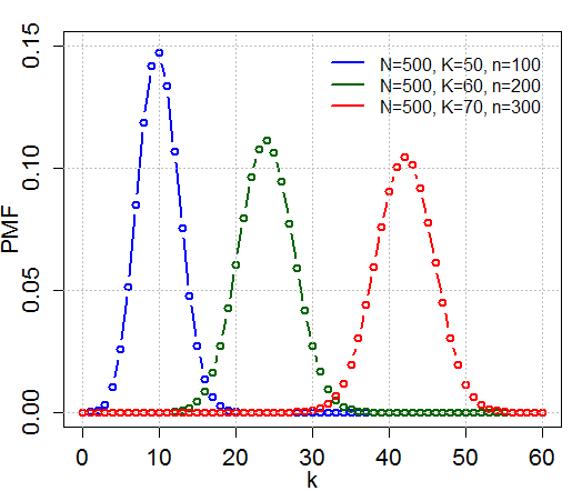
In quality control processes, the hypergeometric distribution quantifies the probability of encountering a specific number of defective items when sampling without replacement from a finite production batch, accounting for the depletion of the population that alters successive draw probabilities unlike independent trials in binomial models.[36] For example, consider a factory producing 1,000 widgets where quality assurance reveals K=50 defectives prior to full shipment; inspectors then draw n=100 widgets randomly without replacement to evaluate the lot. The random variable X representing observed defectives follows Hypergeometric(N=1000, K=50, n=100), with P(X=k) = [C(50,k) * C(950,100-k)] / C(1000,100), enabling calculation of risks such as P(X ≥ 10) to inform acceptance thresholds that balance false positives and negatives in lot disposition.[37] This interpretation underscores the distribution's utility in finite-population scenarios where sampling fraction n/N exceeds typical binomial approximations (e.g., here ~10%), as dependencies inflate variance relative to np(1-p).[38] In electoral auditing, the hypergeometric distribution interprets the consistency between sampled ballots and aggregate tallies to detect irregularities in finite vote universes without replacement assumptions.[39] For instance, in a jurisdiction with N=10,000 ballots where K=6,000 validly favor Candidate A per official count, auditors might hand-recount n=500 randomly selected ballots, modeling X=observed A votes as Hypergeometric(N=10,000, K=6,000, n=500); deviations like P(X ≤ 240) could signal fraud probabilities under null hypotheses of accurate reporting, guiding risk-limiting audits that scale sample sizes inversely with desired error bounds.[40] Such applications highlight causal dependencies in vote pools, where early discrepancies propagate evidential weight, prioritizing empirical verification over approximations valid only for negligible sampling fractions.[41]Statistical Inference
Point and Interval Estimation
The method of moments provides a straightforward point estimator for the success proportion , given by the sample proportion . This follows from equating the observed mean to the theoretical expectation , yielding an unbiased estimator since . The corresponding estimator for is , which is rounded to the nearest integer when must be integral.[42] The maximum likelihood estimator (MLE) for maximizes the hypergeometric probability mass function over integer values of between wait, and , but typically from 0 to N. Computation involves finding the where the likelihood ratio , with . For large and , the MLE approximates the method of moments estimator but incorporates discreteness effects, often computed numerically or via software implementing recursive evaluation. In related capture-recapture contexts modeled by the hypergeometric distribution, bias-reduced MLE variants like (floored if necessary) are used, though exact form requires case-specific verification.[43][44] Interval estimation for or accounts for the variance , which includes a finite population correction factor . An approximate confidence interval for is , where is the quantile of the standard normal distribution; this performs well when and is not too small relative to . For , the interval is times the one for , clipped to integers [0, N].[42] Exact confidence intervals, preferred for small samples to achieve nominal coverage despite discreteness, are constructed by inverting hypergeometric tests: the interval for comprises all integers such that the two-sided p-value for testing given observed exceeds , computed as . Efficient algorithms using tail probability recursions enable fast computation without full enumeration, yielding shortest intervals with guaranteed coverage at least . These methods outperform approximations in finite samples and are implemented in statistical software.[45][46]Hypothesis Testing with Fisher's Exact Test
Fisher's exact test utilizes the hypergeometric distribution to conduct precise hypothesis testing for independence between two dichotomous variables represented in a 2×2 contingency table, particularly suitable for small sample sizes where asymptotic approximations like the chi-squared test fail.[47] The test conditions on the observed row and column marginal totals, treating one cell entry—such as the count of successes in the first group—as a realization from a hypergeometric distribution with population size equal to the grand total, as the total successes in the population, and as the sample size from the first group.[48] Under the null hypothesis of independence (equivalent to an odds ratio of 1), this conditional distribution holds exactly, without reliance on large-sample assumptions.[49] The probability mass function for the hypergeometric random variable (representing the cell count) is given by , where ranges from to .[48] To compute the p-value, all possible tables with the fixed margins are enumerated, each assigned a hypergeometric probability, and the p-value is the sum of probabilities for tables at least as extreme as the observed one. For a two-sided test, this typically includes tables with probabilities less than or equal to that of the observed table; one-sided variants sum over the tail in the direction of the alternative hypothesis.[48] [49] This approach ensures the test maintains its nominal significance level exactly, even with sparse data where more than 20% of expected cell frequencies are below 5 or any below 1, conditions under which the chi-squared test's approximation is unreliable.[47] For instance, in analyzing whether a treatment affects binary outcomes across two groups, the test evaluates evidence against the null by quantifying the rarity of the observed association under hypergeometric sampling.[49] Computational implementation often involves software like R'sfisher.test() function, which handles enumeration directly for moderate sizes or simulation for larger ones.[48]