Ray casting is the most basic of many computer graphics rendering algorithms that use the geometric algorithm of ray tracing. Ray tracing-based rendering algorithms operate in image order to render three-dimensional scenes to two-dimensional images. Geometric rays are traced from the eye of the observer to sample the light (radiance) travelling toward the observer from the ray direction. The speed and simplicity of ray casting comes from computing the color of the light without recursively tracing additional rays that sample the radiance incident on the point that the ray hit. This eliminates the possibility of accurately rendering reflections, refractions, or the natural falloff of shadows; however all of these elements can be faked to a degree, by creative use of texture maps or other methods. The high speed of calculation made ray casting a handy rendering method in early real-time 3D video games.

The idea behind ray casting is to trace rays from the eye, one per pixel, and find the closest object blocking the path of that ray—think of an image as a screen-door, with each square in the screen being a pixel. This is then the object the eye sees through that pixel. Using the material properties and the effect of the lights in the scene, this algorithm can determine the shading of this object. The simplifying assumption is made that if a surface faces a light, the light will reach that surface and not be blocked or in shadow. The shading of the surface is computed using traditional 3D computer graphics shading models. One important advantage ray casting offered over older scanline algorithms was its ability to easily deal with non-planar surfaces and solids, such as cones and spheres. If a mathematical surface can be intersected by a ray, it can be rendered using ray casting. Elaborate objects can be created by using solid modelling techniques and easily rendered.

From the abstract for the paper "Ray Casting for Modeling Solids":^[5]

To visualize and analyze the composite solids modeled, virtual light rays are cast as probes. By virtue of its simplicity, ray casting is reliable and extensible. The most difficult mathematical problem is finding line-surface intersection points. So, surfaces as planes, quadrics, tori, and probably even parametric surface patches may bound the primitive solids. The adequacy and efficiency of ray casting are issues addressed here. A fast picture generation capability for interactive modeling is the biggest challenge.

Light rays and the camera geometry form the basis for all geometric reasoning here. This figure shows a pinhole camera model for perspective effect in image processing and a parallel camera model for mass analysis. The simple pinhole camera model consists of a focal point (or eye point) and a square pixel array (or screen). Straight light rays pass through the pixel array to connect the focal point with the scene, one ray per pixel. To shade pictures, the rays’ intensities are measured and stored as pixels. The reflecting surface responsible for a pixel’s value intersects the pixel’s ray.

When the focal length, distance between focal point and screen, is infinite, then the view is called “parallel” because all light rays are parallel to each other, perpendicular to the screen. Although the perspective view is natural for making pictures, some applications need rays that can be uniformly distributed in space.

For modeling convenience, a typical standard coordinate system for the camera has the screen in the X–Y plane, the scene in the +Z half space, and the focal point on the −Z axis.

A ray is simply a straight line in the 3D space of the camera model. It is best defined in parameterized form as a point vector (X₀, Y₀, Z₀) and a direction vector (D_x, D_y, D_z). In this form, points on the line are ordered and accessed via a single parameter t. For every value of t, a corresponding point (X, Y, Z) on the line is defined:

X = X0 + t · Dx
Y = Y0 + t · Dy
Z = Z0 + t · Dz

If the vector is normalized, then the parameter t is distance along the line. The vector can be normalized easily with the following computation:

Dist = √(Dx2 + Dy2 + Dz2)
D'x = Dx / Dist
D'y = Dy / Dist
D'z = Dz / Dist

Given geometric definitions of the objects, each bounded by one or more surfaces, the result of computing one ray’s intersection with all bounded surfaces in the screen is defined by two arrays:

Ray parameters:   t[1], t[2], …, t[n]
Surface pointers: S[1], S[2], …, S[n]

Where n is the number of ray-surface intersections. The ordered list of ray parameters, t[i], denote the enter–exit points. The ray enters a solid at point t[1], exits at t[2], enters a solid at t[3], etc. Point t[1] is closest to the camera and t[n] is furthest.

In association with the ray parameters, the surface pointers contain a unique address for the intersected surface’s information. The surface can have various properties such as color, specularity, transparency with/without refraction, translucency, etc. The solid associated with the surface may have its own physical properties such as density. This could be useful, for instance, when an object consists of an assembly of different materials and the overall center of mass and moments of inertia are of interest.

Three algorithms using ray casting are to make line drawings, to make shaded pictures, and to compute volumes and other physical properties. Each algorithm, given a camera model, casts one ray per pixel in the screen. For computing volume, the resolution of the pixel screen to use depends on the desired accuracy of the solution. For line drawings and picture shading, the resolution determines the quality of the image.

To draw the visible edges of a solid, generate one ray per pixel moving top-down, left-right in the screen. Evaluate each ray in order to identify the visible surface S[1], the first surface pointer in the sorted list of ray-surface intersections. If the visible surface at pixel location (X, Y) is different than the visible surface at pixel (X−1, Y), then display a vertical line one pixel long centered at (X−½, Y). Similarly, if the visible surface at (X, Y) is different than the visible surface at pixel (X, Y−1), then display a horizontal line one pixel long centered at (X, Y−½). The resulting drawing will consist of horizontal and vertical edges only, looking jagged in coarse resolutions.

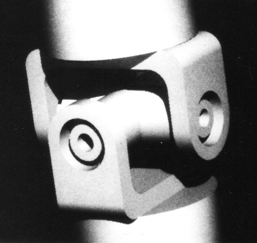
Roth’s ray casting system generated the images of solid objects on the right. Box enclosures, dynamic bounding, and coherence were used for optimization. For each picture, the screen was sampled with a density of about 100×100 (e.g., 10,000) rays and new edges were located via binary searches. Then all edges were followed by casting additional rays at one pixel increments on the two sides of the edges. Each picture was drawn on a Tektronix tube at 780×780 resolution.

To make a shaded picture, again cast one ray per pixel in the screen. This time, however, use the visible surface pointer S[1] at each pixel to access the description of the surface. From this, compute the surface normal at the visible point t[1]. The pixel’s value, the displayable light intensity, is proportional to the cosine of the angle formed by the surface normal and the light-source-to-surface vector. Processing all pixels this way produces a raster-type picture of the scene.

The volume (and similar properties) of a solid bounded by curved surfaces is easily computed by the “approximating sums” integration method, by approximating the solid with a set of rectangular parallelepipeds. This is accomplished by taking an “in-depth” picture of the solid in a parallel view. Casting rays through the screen into the solid partitions the solid into volume elements. Two dimensions of the parallelepipeds are constant, defined by the 2D spacing of rays in the screen. The third dimension is variable, defined by the enter–exit point computed. Specifically, if the horizontal and vertical distances between rays in the screen is S, then the volume “detected” by each ray is:

S × S ×  (t[2]-t[1]  +  t[4]-t[3]  + … + t[n]-t[n-1]) / L

where L is defined as the length of the direction vector. (If already normalized, this is equal to 1.)

L = √(Dx2 + Dy2 + Dz2)

Each (t[i]-t[i-1])/L is a length of a ray segment that is inside of the solid.

This figure shows the parallelepipeds for a modeled solid using ray casting. This is a use of parallel-projection camera model.

This figure shows an example of the binary operators in a composition tree using “+” and “−” where a single ray is evaluated.

The ray casting procedure starts at the top of the solid composition tree, recursively descends to the bottom, classifies the ray with respect to the primitive solids, and then returns up the tree combining the classifications of the left and right subtrees.

This figure illustrates the combining of the left and right classifications for all three binary operators.

Ray casting is a natural modeling tool for making shaded pictures. The grayscale ray-casting system developed by Scott Roth and Daniel Bass at GM Research Labs produced pictures on a Ramtek color raster display around 1979. To compose pictures, the system provided the user with the following controls:

• View
  • Viewing direction and position
  • Focal length: width-angle perspective to parallel
  • Zoom factor
• Illumination
  • Number of light sources
  • Locations and intensities of lights
  • Optionally shadow
  • Intensities of ambient light and background
• Surface reflectance
  • % reflected diffusely
  • % reflected specularly
  • % transmitted

This figure shows a table scene with shadows from two point light sources.

Shading algorithms that implement all of the realistic effects are computationally expensive, but relatively simple. For example, the following figure shows the additional rays that could be cast for a single light source.

For a single pixel in the image to be rendered, the algorithm casts a ray starting at the focal point and determines that it intersects a semi-transparent rectangle and a shiny circle. An additional ray must then be cast starting at that point in the direction symmetrically opposite the surface normal at the ray-surface intersection point in order to determine what is visible in the mirrored reflection. That ray intersects the triangle which is opaque. Finally, each ray-surface intersection point is tested to determine if it is in shadow. The “Shadow feeler” ray is cast from the ray-surface intersection point to the light source to determine if any other surface blocks that pathway.

Turner Whitted calls the secondary and additional rays “Recursive Ray Tracing”.^[6] [A room of mirrors would be costly to render, so limiting the number of recursions is prudent.] Whitted modeled refraction for transparencies by generating a secondary ray from the visible surface point at an angle determined by the solid’s index of refraction. The secondary ray is then processed as a specular ray. For the refraction formula and pictorial examples, see Whitted’s paper.

Ray casting qualifies as a brute force method for solving problems. The minimal algorithm is simple, particularly in consideration of its many applications and ease of use, but applications typically cast many rays. Millions of rays may be cast to render a single frame of an animated film. Computer processing time increases with the resolution of the screen and the number of primitive solids/surfaces in the composition.

By using minimum bounding boxes around the solids in the composition tree, the exhaustive search for a ray-solid intersection resembles an efficient binary search. The brute force algorithm does an exhaustive search because it always visits all the nodes in the tree—transforming the ray into primitives’ local coordinate systems, testing for ray-surface intersections, and combining the classifications—even when the ray clearly misses the solid. In order to detect a “clear miss”, a faster algorithm uses the binary composition tree as a hierarchical representation of the space that the solid composition occupies. But all position, shape, and size information is stored at the leaves of the tree where primitive solids reside. The top and intermediate nodes in the tree only specify combine operators.

Characterizing with enclosures the space that all solids fill gives all nodes in the tree an abstract summary of position and size information. Then, the quick “ray intersects enclosure” tests guide the search in the hierarchy. When the test fails at an intermediate node in the tree, the ray is guaranteed to classify as out of the composite, so recursing down its subtrees to further investigate is unnecessary.

Accurately assessing the cost savings for using enclosures is difficult because it depends on the spatial distribution of the primitives (the complexity distribution) and on the organization of the composition tree. The optimal conditions are:

• No primitive enclosures overlap in space
• Composition tree is balanced and organized so that sub-solids near in space are also nearby in the tree

In contrast, the worst condition is:

• All primitive enclosures mutually overlap

The following are miscellaneous performance improvements made in Roth’s paper on ray casting, but there have been considerable improvements subsequently made by others.

Early Outs

If the operator at a composite node in the tree is − or & and the ray classifies as out of the composite’s left sub-solid, then the ray will classify as out of the composite regardless of the ray’s classification with respect to the right sub-solid. So, classifying the ray with respect to the right sub-solid is unnecessary and should be avoided for efficiency.

Transformations

By initially combining the screen-to-scene transform with the primitive’s scene-to-local transform and storing the resulting screen-to-local transforms in the primitive’s data structures, one ray transform per ray-surface intersection is eliminated.

Recursion

Given a deep composition tree, recursion can be expensive in combination with allocating and freeing up memory. Recursion can be simulated using static arrays as stacks.

Dynamic Bounding

If only the visible edges of the solid are to be displayed, the ray casting algorithm can dynamically bound the ray to cut off the search. That is, after finding that a ray intersects a sub-solid, the algorithm can use the intersection point closest to the screen to tighten the depth bound for the “ray intersections box” test. This only works for the + part of the tree, starting at the top. With – and &, nearby “in” parts of the ray may later become “out”.

Coherence

The principle of coherence is that the surfaces visible at two neighboring pixels are more likely to be the same than different. Developers of computer graphics and vision systems have applied this empirical truth for efficiency and performance. For line drawings, the image area containing edges is normally much less than the total image area, so ray casting should be concentrated around the edges and not in the open regions. This can be effectively implemented by sparsely sampling the screen with rays and then locating, when neighboring rays identify different visible surfaces, the edges via binary searches.

The jagged edges caused by aliasing is an undesirable effect of point sampling techniques and is a classic problem with raster display algorithms. Linear or smoothly curved edges will appear jagged and are particularly objectionable in animations because movement of the image makes the edges appear fuzzy or look like little moving escalators. Also, details in the scene smaller than the spacing between rays may be lost. The jagged edges in a line drawing can be smoothed by edge following. The purpose of such an algorithm is to minimize the number of lines needed to draw the picture within one pixel accuracy. Smooth edges result. The line drawings above were drawn this way.

To smooth the jagged edges in a shaded picture with subpixel accuracy, additional rays should be cast for information about the edges. (See Supersampling for a general approach.) Edges are formed by the intersection of surfaces or by the profile of a curved surface. Applying "Coherence" as described above via binary search, if the visible surface at pixel (X,Y) is different than the visible surface at pixel (X+1,Y), then a ray could be generated midway between them at (X+½,Y) and the visible surface there identified. The distance between sample points could be further subdivided, but the search need not be deep. The primary search depth to smooth jagged edges is a function of the intensity gradient across the edge. The cost for smoothing jagged edges is affordable, since:

• the area of the image that contains edges is usually a small percentage of the total area; and
• the extra rays cast in binary searches can be bounded in depth (that of the visible primitives forming the edges).

For the history of ray casting, see Ray tracing (graphics) as both are essentially the same technique under different names. Scott Roth had invented the term "ray casting" before having heard of "ray tracing". Additionally, Scott Roth's development of ray casting at GM Research Labs occurred concurrently with Turner Whitted's ray tracing work at Bell Labs.

In early first person games, raycasting was used to efficiently render a 3D world from a 2D playing field using a simple one-dimensional scan over the horizontal width of the screen.^[7] Early first-person shooters used 2D ray casting as a technique to create a 3D effect from a 2D world. While the world appears 3D, the player cannot look up or down or only in limited angles with shearing distortion.^[7][8] This style of rendering eliminates the need to fire a ray for each pixel in the frame as is the case with modern engines; once the hit point is found the projection distortion is applied to the surface texture and an entire vertical column is copied from the result into the frame. This style of rendering also imposes limitations on the type of rendering which can be performed, for example depth sorting but depth buffering may not. That is polygons must be full in front of or behind one another, they may not partially overlap or intersect.

The video game Wolfenstein 3D was built from a square based grid of uniform height walls meeting solid-colored floors and ceilings. In order to draw the world, a single ray was traced for every column of screen pixels and a vertical slice of wall texture was selected and scaled according to where in the world the ray hits a wall and how far it travels before doing so.^[9]

The purpose of the grid based levels was twofold — ray-wall collisions can be found more quickly since the potential hits become more predictable and memory overhead is reduced. However, encoding wide-open areas takes extra space.

The Raven Software game ShadowCaster uses an improved Wolfenstein-based engine with added floors and ceilings texturing and variable wall heights.

The Voxel Space engine developed by NovaLogic for the Comanche games traced a ray through each column of screen pixels and tested each ray against points in a heightmap. Then it transformed each element of the heightmap into a column of pixels, determined which are visible (that is, have not been occluded by pixels that have been drawn in front), and drew them with the corresponding color from the texture map.^[10]

Later DOS games like id Software's DOOM kept many of the raycasting 2.5D restrictions for speed but went on to switch to alternative rendering techniques (like BSP), making them no longer raycasting engines.^[11]

This section needs expansion. You can help by adding to it. (May 2010)

In computational geometry, the ray casting problem is also known as the ray shooting problem and may be stated as the following query problem: given a set of objects in d-dimensional space, preprocess them into a data structure so that for each query ray, the initial object hit by the ray can be found quickly. The problem has been investigated for various settings: space dimension, types of objects, restrictions on query rays, etc.^[12] One technique is to use a sparse voxel octree.

• Ray tracing (graphics) A more sophisticated ray-casting algorithm which considers global illumination
• Photon mapping
• Radiosity (computer graphics)
• Path tracing
• Volume ray casting
• 2.5D