Scale space

The notion of scale space applies to signals of arbitrary numbers of variables. The most common case in the literature applies to two-dimensional images, which is what is presented here. Consider a given image ${\displaystyle f}$ where ${\displaystyle f(x,y)}$ is the greyscale value of the pixel at position ${\displaystyle (x,y)}$. The linear (Gaussian) scale-space representation of ${\displaystyle f}$ is a family of derived signals ${\displaystyle L(x,y;t)}$ defined by the convolution of ${\displaystyle f(x,y)}$ with the two-dimensional Gaussian kernel

${\displaystyle g(x,y;t)={\frac {1}{2\pi t}}e^{-(x^{2}+y^{2})/2t}\,}$

such that

${\displaystyle L(\cdot ,\cdot ;t)\ =g(\cdot ,\cdot ;t)*f(\cdot ,\cdot ),}$

where the semicolon in the argument of ${\displaystyle L}$ implies that the convolution is performed only over the variables ${\displaystyle x,y}$, while the scale parameter ${\displaystyle t}$ after the semicolon just indicates which scale level is being defined. This definition of ${\displaystyle L}$ works for a continuum of scales ${\displaystyle t\geq 0}$, but typically only a finite discrete set of levels in the scale-space representation would be actually considered.

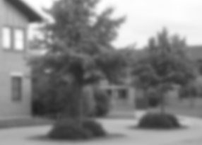
The scale parameter ${\displaystyle t=\sigma ^{2}}$ is the variance of the Gaussian filter and as a limit for ${\displaystyle t=0}$ the filter ${\displaystyle g}$ becomes an impulse function such that ${\displaystyle L(x,y;0)=f(x,y),}$ that is, the scale-space representation at scale level ${\displaystyle t=0}$ is the image ${\displaystyle f}$ itself. As ${\displaystyle t}$ increases, ${\displaystyle L}$ is the result of smoothing ${\displaystyle f}$ with a larger and larger filter, thereby removing more and more of the details that the image contains. Since the standard deviation of the filter is ${\displaystyle \sigma ={\sqrt {t}}}$, details that are significantly smaller than this value are to a large extent removed from the image at scale parameter ${\displaystyle t}$, see the following figures and^[11] for graphical illustrations.

• 
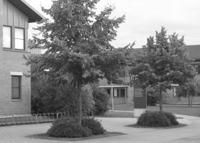  Scale-space representation ${\displaystyle L(x,y;t)}$ at scale ${\displaystyle t=0}$, corresponding to the original image ${\displaystyle f}$
• 
  Scale-space representation ${\displaystyle L(x,y;t)}$ at scale ${\displaystyle t=1}$
• 
  Scale-space representation ${\displaystyle L(x,y;t)}$ at scale ${\displaystyle t=4}$
• 
  Scale-space representation ${\displaystyle L(x,y;t)}$ at scale ${\displaystyle t=16}$
• 
  Scale-space representation ${\displaystyle L(x,y;t)}$ at scale ${\displaystyle t=64}$
• 
  Scale-space representation ${\displaystyle L(x,y;t)}$ at scale ${\displaystyle t=256}$

When faced with the task of generating a multi-scale representation one may ask: could any filter g of low-pass type and with a parameter t which determines its width be used to generate a scale space? The answer is no, as it is of crucial importance that the smoothing filter does not introduce new spurious structures at coarse scales that do not correspond to simplifications of corresponding structures at finer scales. In the scale-space literature, a number of different ways have been expressed to formulate this criterion in precise mathematical terms.

The conclusion from several different axiomatic derivations that have been presented is that the Gaussian scale space constitutes the canonical way to generate a linear scale space, based on the essential requirement that new structures must not be created when going from a fine scale to any coarser scale.^{[1][3][4][6][9][12][13][14][15][16][17][18][19]} Conditions, referred to as scale-space axioms, that have been used for deriving the uniqueness of the Gaussian kernel include linearity, shift invariance, semi-group structure, non-enhancement of local extrema, scale invariance and rotational invariance. In the works,^[15][20][21] the uniqueness claimed in the arguments based on scale invariance has been criticized, and alternative self-similar scale-space kernels have been proposed. The Gaussian kernel is, however, a unique choice according to the scale-space axiomatics based on causality^[3] or non-enhancement of local extrema.^[16][18]

Equivalently, the scale-space family can be defined as the solution of the diffusion equation (for example in terms of the heat equation),

${\displaystyle \partial _{t}L={\frac {1}{2}}\nabla ^{2}L,}$

with initial condition ${\displaystyle L(x,y;0)=f(x,y)}$. This formulation of the scale-space representation L means that it is possible to interpret the intensity values of the image f as a "temperature distribution" in the image plane and that the process that generates the scale-space representation as a function of t corresponds to heat diffusion in the image plane over time t (assuming the thermal conductivity of the material equal to the arbitrarily chosen constant ⁠1/2⁠). Although this connection may appear superficial for a reader not familiar with differential equations, it is indeed the case that the main scale-space formulation in terms of non-enhancement of local extrema is expressed in terms of a sign condition on partial derivatives in the 2+1-D volume generated by the scale space, thus within the framework of partial differential equations. Furthermore, a detailed analysis of the discrete case shows that the diffusion equation provides a unifying link between continuous and discrete scale spaces, which also generalizes to nonlinear scale spaces, for example, using anisotropic diffusion. Hence, one may say that the primary way to generate a scale space is by the diffusion equation, and that the Gaussian kernel arises as the Green's function of this specific partial differential equation.

The motivation for generating a scale-space representation of a given data set originates from the basic observation that real-world objects are composed of different structures at different scales. This implies that real-world objects, in contrast to idealized mathematical entities such as points or lines, may appear in different ways depending on the scale of observation. For example, the concept of a "tree" is appropriate at the scale of meters, while concepts such as leaves and molecules are more appropriate at finer scales. For a computer vision system analysing an unknown scene, there is no way to know a priori what scales are appropriate for describing the interesting structures in the image data. Hence, the only reasonable approach is to consider descriptions at multiple scales in order to be able to capture the unknown scale variations that may occur. Taken to the limit, a scale-space representation considers representations at all scales.^[9]

Another motivation to the scale-space concept originates from the process of performing a physical measurement on real-world data. In order to extract any information from a measurement process, one has to apply operators of non-infinitesimal size to the data. In many branches of computer science and applied mathematics, the size of the measurement operator is disregarded in the theoretical modelling of a problem. The scale-space theory on the other hand explicitly incorporates the need for a non-infinitesimal size of the image operators as an integral part of any measurement as well as any other operation that depends on a real-world measurement.^[5]

There is a close link between scale-space theory and biological vision. Many scale-space operations show a high degree of similarity with receptive field profiles recorded from the mammalian retina and the first stages in the visual cortex. In these respects, the scale-space framework can be seen as a theoretically well-founded paradigm for early vision, which in addition has been thoroughly tested by algorithms and experiments.^[4][9]

At any scale in scale space, we can apply local derivative operators to the scale-space representation:

${\displaystyle L_{x^{m}y^{n}}(x,y;t)=\left(\partial _{x^{m}y^{n}}L\right)(x,y;t).}$

Due to the commutative property between the derivative operator and the Gaussian smoothing operator, such scale-space derivatives can equivalently be computed by convolving the original image with Gaussian derivative operators. For this reason they are often also referred to as Gaussian derivatives:

${\displaystyle L_{x^{m}y^{n}}(\cdot ,\cdot ;t)=\partial _{x^{m}y^{n}}g(\cdot ,\cdot ;\,t)*f(\cdot ,\cdot ).}$

The uniqueness of the Gaussian derivative operators as local operations derived from a scale-space representation can be obtained by similar axiomatic derivations as are used for deriving the uniqueness of the Gaussian kernel for scale-space smoothing.^[4][22]

These Gaussian derivative operators can in turn be combined by linear or non-linear operators into a larger variety of different types of feature detectors, which in many cases can be well modelled by differential geometry. Specifically, invariance (or more appropriately covariance) to local geometric transformations, such as rotations or local affine transformations, can be obtained by considering differential invariants under the appropriate class of transformations or alternatively by normalizing the Gaussian derivative operators to a locally determined coordinate frame determined from e.g. a preferred orientation in the image domain, or by applying a preferred local affine transformation to a local image patch (see the article on affine shape adaptation for further details).

When Gaussian derivative operators and differential invariants are used in this way as basic feature detectors at multiple scales, the uncommitted first stages of visual processing are often referred to as a visual front-end. This overall framework has been applied to a large variety of problems in computer vision, including feature detection, feature classification, image segmentation, image matching, motion estimation, computation of shape cues and object recognition. The set of Gaussian derivative operators up to a certain order is often referred to as the N-jet and constitutes a basic type of feature within the scale-space framework.

Following the idea of expressing visual operations in terms of differential invariants computed at multiple scales using Gaussian derivative operators, we can express an edge detector from the set of points that satisfy the requirement that the gradient magnitude

${\displaystyle L_{v}={\sqrt {L_{x}^{2}+L_{y}^{2}}}}$

should assume a local maximum in the gradient direction

${\displaystyle \nabla L=(L_{x},L_{y})^{T}.}$

By working out the differential geometry, it can be shown ^[4] that this differential edge detector can equivalently be expressed from the zero-crossings of the second-order differential invariant

${\displaystyle {\tilde {L}}_{v}^{2}=L_{x}^{2}\,L_{xx}+2\,L_{x}\,L_{y}\,L_{xy}+L_{y}^{2}\,L_{yy}=0}$

that satisfy the following sign condition on a third-order differential invariant:

${\displaystyle {\tilde {L}}_{v}^{3}=L_{x}^{3}\,L_{xxx}+3\,L_{x}^{2}\,L_{y}\,L_{xxy}+3\,L_{x}\,L_{y}^{2}\,L_{xyy}+L_{y}^{3}\,L_{yyy}<0.}$

Similarly, multi-scale blob detectors at any given fixed scale^[23][9] can be obtained from local maxima and local minima of either the Laplacian operator (also referred to as the Laplacian of Gaussian)

${\displaystyle \nabla ^{2}L=L_{xx}+L_{yy}\,}$

or the determinant of the Hessian matrix

${\displaystyle \operatorname {det} HL(x,y;t)=(L_{xx}L_{yy}-L_{xy}^{2}).}$

In an analogous fashion, corner detectors and ridge and valley detectors can be expressed as local maxima, minima or zero-crossings of multi-scale differential invariants defined from Gaussian derivatives. The algebraic expressions for the corner and ridge detection operators are, however, somewhat more complex and the reader is referred to the articles on corner detection and ridge detection for further details.

Scale-space operations have also been frequently used for expressing coarse-to-fine methods, in particular for tasks such as image matching and for multi-scale image segmentation.

The theory presented so far describes a well-founded framework for representing image structures at multiple scales. In many cases it is, however, also necessary to select locally appropriate scales for further analysis. This need for scale selection originates from two major reasons; (i) real-world objects may have different size, and this size may be unknown to the vision system, and (ii) the distance between the object and the camera can vary, and this distance information may also be unknown a priori. A highly useful property of scale-space representation is that image representations can be made invariant to scales, by performing automatic local scale selection^{[9][10][23][24][25][26][27][28]} based on local maxima (or minima) over scales of scale-normalized derivatives

${\displaystyle L_{\xi ^{m}\eta ^{n}}(x,y;t)=t^{(m+n)\gamma /2}L_{x^{m}y^{n}}(x,y;t)}$

where ${\displaystyle \gamma \in [0,1]}$ is a parameter that is related to the dimensionality of the image feature. This algebraic expression for scale normalized Gaussian derivative operators originates from the introduction of ${\displaystyle \gamma }$-normalized derivatives according to

${\displaystyle \partial _{\xi }=t^{\gamma /2}\partial _{x}\quad }$ and ${\displaystyle \quad \partial _{\eta }=t^{\gamma /2}\partial _{y}.}$

It can be theoretically shown that a scale selection module working according to this principle will satisfy the following scale covariance property: if for a certain type of image feature a local maximum is assumed in a certain image at a certain scale ${\displaystyle t_{0}}$, then under a rescaling of the image by a scale factor ${\displaystyle s}$ the local maximum over scales in the rescaled image will be transformed to the scale level ${\displaystyle s^{2}t_{0}}$.^[23]

Following this approach of gamma-normalized derivatives, it can be shown that different types of scale adaptive and scale invariant feature detectors^{[9][10][23][24][25][29][30][27]} can be expressed for tasks such as blob detection, corner detection, ridge detection, edge detection and spatio-temporal interest point detection (see the specific articles on these topics for in-depth descriptions of how these scale-invariant feature detectors are formulated). Furthermore, the scale levels obtained from automatic scale selection can be used for determining regions of interest for subsequent affine shape adaptation^[31] to obtain affine invariant interest points^[32][33] or for determining scale levels for computing associated image descriptors, such as locally scale adapted N-jets.

Recent work has shown that also more complex operations, such as scale-invariant object recognition can be performed in this way, by computing local image descriptors (N-jets or local histograms of gradient directions) at scale-adapted interest points obtained from scale-space extrema of the normalized Laplacian operator (see also scale-invariant feature transform^[34]) or the determinant of the Hessian (see also SURF);^[35] see also the Scholarpedia article on the scale-invariant feature transform^[36] for a more general outlook of object recognition approaches based on receptive field responses^{[19][37][38][39]} in terms Gaussian derivative operators or approximations thereof.

An image pyramid is a discrete representation in which a scale space is sampled in both space and scale. For scale invariance, the scale factors should be sampled exponentially, for example as integer powers of 2 or √2. When properly constructed, the ratio of the sample rates in space and scale are held constant so that the impulse response is identical in all levels of the pyramid.^{[40][41][42][43]} Fast, O(N), algorithms exist for computing a scale invariant image pyramid, in which the image or signal is repeatedly smoothed then subsampled. Values for scale space between pyramid samples can easily be estimated using interpolation within and between scales and allowing for scale and position estimates with sub resolution accuracy.^[43]

In a scale-space representation, the existence of a continuous scale parameter makes it possible to track zero crossings over scales leading to so-called deep structure. For features defined as zero-crossings of differential invariants, the implicit function theorem directly defines trajectories across scales,^[4][44] and at those scales where bifurcations occur, the local behaviour can be modelled by singularity theory.^{[4][44][45][46][47]}

Extensions of linear scale-space theory concern the formulation of non-linear scale-space concepts more committed to specific purposes.^[48][49] These non-linear scale-spaces often start from the equivalent diffusion formulation of the scale-space concept, which is subsequently extended in a non-linear fashion. A large number of evolution equations have been formulated in this way, motivated by different specific requirements (see the abovementioned book references for further information). However, not all of these non-linear scale-spaces satisfy similar "nice" theoretical requirements as the linear Gaussian scale-space concept. Hence, unexpected artifacts may sometimes occur and one should be very careful of not using the term "scale-space" for just any type of one-parameter family of images.

A first-order extension of the isotropic Gaussian scale space is provided by the affine (Gaussian) scale space.^[4] One motivation for this extension originates from the common need for computing image descriptors subject for real-world objects that are viewed under a perspective camera model. To handle such non-linear deformations locally, partial invariance (or more correctly covariance) to local affine deformations can be achieved by considering affine Gaussian kernels with their shapes determined by the local image structure,^[31] see the article on affine shape adaptation for theory and algorithms. Indeed, this affine scale space can also be expressed from a non-isotropic extension of the linear (isotropic) diffusion equation, while still being within the class of linear partial differential equations.

There exists a more general extension of the Gaussian scale-space model to affine and spatio-temporal scale-spaces.^{[4][31][18][19][50]} In addition to variabilities over scale, which original scale-space theory was designed to handle, this generalized scale-space theory^[19] also comprises other types of variabilities caused by geometric transformations in the image formation process, including variations in viewing direction approximated by local affine transformations, and relative motions between objects in the world and the observer, approximated by local Galilean transformations. This generalized scale-space theory leads to predictions about receptive field profiles in good qualitative agreement with receptive field profiles measured by cell recordings in biological vision.^{[51][52][50][53]}

There are strong relations between scale-space theory and wavelet theory, although these two notions of multi-scale representation have been developed from somewhat different premises. There has also been work on other multi-scale approaches, such as pyramids and a variety of other kernels, that do not exploit or require the same requirements as true scale-space descriptions do.

There are interesting relations between scale-space representation and biological vision and hearing. Neurophysiological studies of biological vision have shown that there are receptive field profiles in the mammalian retina and visual cortex, that can be well modelled by linear Gaussian derivative operators, in some cases also complemented by a non-isotropic affine scale-space model, a spatio-temporal scale-space model and/or non-linear combinations of such linear operators.^{[18][51][52][50][53][54][55][56][57]}

Regarding biological hearing there are receptive field profiles in the inferior colliculus and the primary auditory cortex that can be well modelled by spectra-temporal receptive fields that can be well modelled by Gaussian derivates over logarithmic frequencies and windowed Fourier transforms over time with the window functions being temporal scale-space kernels.^[58][59]

In the area of classical computer vision, scale-space theory has established itself as a theoretical framework for early vision, with Gaussian derivatives constituting a canonical model for the first layer of receptive fields. With the introduction of deep learning, there has also been work on also using Gaussian derivatives or Gaussian kernels as a general basis for receptive fields in deep networks.^{[60][61][62][63][64]} Using the transformation properties of the Gaussian derivatives and Gaussian kernels under scaling transformations, it is in this way possible to obtain scale covariance/equivariance and scale invariance of the deep network to handle image structures at different scales in a theoretically well-founded manner.^[62][63] There have also been approaches developed to obtain scale covariance/equivariance and scale invariance by learned filters combined with multiple scale channels.^{[65][66][67][68][69][70]} Specifically, using the notions of scale covariance/equivariance and scale invariance, it is possible to make deep networks operate robustly at scales not spanned by the training data, thus enabling scale generalization.^{[62][63][67][69]}

For processing pre-recorded temporal signals or video, the Gaussian kernel can also be used for smoothing and suppressing fine-scale structures over the temporal domain, since the data are pre-recorded and available in all directions. When processing temporal signals or video in real-time situations, the Gaussian kernel cannot, however, be used for temporal smoothing, since it would access data from the future, which obviously cannot be available. For temporal smoothing in real-time situations, one can instead use the temporal kernel referred to as the time-causal limit kernel,^[71] which possesses similar properties in a time-causal situation (non-creation of new structures towards increasing scale and temporal scale covariance) as the Gaussian kernel obeys in the non-causal case. The time-causal limit kernel corresponds to convolution with an infinite number of truncated exponential kernels coupled in cascade, with specifically chosen time constants to obtain temporal scale covariance. For discrete data, this kernel can often be numerically well approximated by a small set of first-order recursive filters coupled in cascade, see ^[71] for further details.

For an earlier approach to handling temporal scales in a time-causal way, by performing Gaussian smoothing over a logarithmically transformed temporal axis, however, not having any known memory-efficient time-recursive implementation as the time-causal limit kernel has, see,^[72]

When implementing scale-space smoothing in practice there are a number of different approaches that can be taken in terms of continuous or discrete Gaussian smoothing, implementation in the Fourier domain, in terms of pyramids based on binomial filters that approximate the Gaussian or using recursive filters. More details about this are given in a separate article on scale space implementation.

• Difference of Gaussians
• Gaussian function
• mipmapping