Scoring rule

Consider a sample space ${\displaystyle \Omega }$, a σ-algebra ${\displaystyle {\mathcal {A}}}$ of subsets of ${\displaystyle \Omega }$ and a convex class ${\displaystyle {\mathcal {F}}}$ of probability measures on ${\displaystyle (\Omega ,{\mathcal {A}})}$. A function defined on ${\displaystyle \Omega }$ and taking values in the extended real line, ${\displaystyle {\overline {\mathbb {R} }}=[-\infty ,\infty ]}$, is ${\displaystyle {\mathcal {F}}}$-quasi-integrable if it is measurable with respect to ${\displaystyle {\mathcal {A}}}$ and is quasi-integrable with respect to all ${\displaystyle F\in {\mathcal {F}}}$.

A probabilistic forecast is any probability measure ${\displaystyle F\in {\mathcal {F}}}$. I.e. it is a distribution of potential future observations.

A scoring rule is any extended real-valued function ${\displaystyle \mathbf {S} :{\mathcal {F}}\times \Omega \rightarrow \mathbb {R} }$ such that ${\displaystyle \mathbf {S} (F,\cdot )}$ is ${\displaystyle {\mathcal {F}}}$-quasi-integrable for all ${\displaystyle F\in {\mathcal {F}}}$. ${\displaystyle \mathbf {S} (F,y)}$ represents the loss or penalty when the forecast ${\displaystyle F\in {\mathcal {F}}}$ is issued and the observation ${\displaystyle y\in \Omega }$ materializes.

A point forecast is a functional, i.e. a potentially set-valued mapping ${\displaystyle F\rightarrow T(F)\subseteq \Omega }$.

A scoring function is any real-valued function ${\displaystyle S:\Omega \times \Omega \rightarrow \mathbb {R} }$ where ${\displaystyle S(x,y)}$ represents the loss or penalty when the point forecast ${\displaystyle x\in \Omega }$ is issued and the observation ${\displaystyle y\in \Omega }$ materializes.

Scoring rules ${\displaystyle \mathbf {S} (F,y)}$ and scoring functions ${\displaystyle S(x,y)}$ are negatively (positively) oriented if smaller (larger) values mean better. Here we adhere to negative orientation, hence the association with "loss".

We write for the expected score of a prediction ${\displaystyle F}$ under ${\displaystyle Q\in {\mathcal {F}}}$ as the expected score of the predicted distribution ${\displaystyle F\in {\mathcal {F}}}$, when sampling observations from distribution ${\displaystyle Q}$.

${\displaystyle \mathbb {E} _{Y\sim Q}[S(F,Y)]=\int \mathbf {S} (F,\omega )\mathrm {d} Q(\omega )}$

Many probabilistic forecasting models are training via the sample average score, in which a set of predicted distributions ${\displaystyle F_{1},\ldots ,F_{n}\in {\mathcal {F}}}$ is evaluated against a set of observations ${\displaystyle y_{1},\ldots ,y_{n}\in \Omega }$.

${\displaystyle {\mathcal {L}}={\frac {1}{n}}\sum _{i=1}^{n}S(F_{i},y_{i})}$

Strictly proper scoring rules and strictly consistent scoring functions encourage honest forecasts by maximization of the expected reward: If a forecaster is given a reward of ${\displaystyle -\mathbf {S} (F,y)}$ if ${\displaystyle y}$ realizes (e.g. ${\displaystyle y=rain}$), then the highest expected reward (lowest score) is obtained by reporting the true probability distribution.^[1]

A scoring rule ${\displaystyle \mathbf {S} }$ is proper relative to ${\displaystyle {\mathcal {F}}}$ if (assuming negative orientation) its expected score is minimized when the forecasted distribution matches the distribution of the observation.

${\displaystyle \mathbb {E} _{Y\sim Q}[S(Q,Y)]\leq \mathbb {E} _{Y\sim Q}[S(F,Y)]}$ for all ${\displaystyle F,Q\in {\mathcal {F}}}$.

It is strictly proper if the above equation holds with equality if and only if ${\displaystyle F=Q}$.

A scoring function ${\displaystyle S}$ is consistent for the functional ${\displaystyle T}$ relative to the class ${\displaystyle {\mathcal {F}}}$ if

${\displaystyle \mathbb {E} _{Y\sim F}[S(t,Y)]\leq \mathbb {E} _{Y\sim F}[S(x,Y)]}$ for all ${\displaystyle F\in {\mathcal {F}}}$, all ${\displaystyle t\in T(F)}$ and all ${\displaystyle x\in \Omega }$.

It is strictly consistent if it is consistent and equality in the above equation implies that ${\displaystyle x\in T(F)}$.

An example of probabilistic forecasting is in meteorology where a weather forecaster may give the probability of rain on the next day. One could note the number of times that a 25% probability was quoted, over a long period, and compare this with the actual proportion of times that rain fell. If the actual percentage was substantially different from the stated probability we say that the forecaster is poorly calibrated. A poorly calibrated forecaster might be encouraged to do better by a bonus system. A bonus system designed around a proper scoring rule will incentivize the forecaster to report probabilities equal to his personal beliefs.^[3]

In addition to the simple case of a binary decision, such as assigning probabilities to 'rain' or 'no rain', scoring rules may be used for multiple classes, such as 'rain', 'snow', or 'clear', or continuous responses like the amount of rain per day.

The image shows an example of a scoring rule, the logarithmic scoring rule, as a function of the probability reported for the event that actually occurred. One way to use this rule would be as a cost based on the probability that a forecaster or algorithm assigns, then checking to see which event actually occurs.

Scoring rules can be used beyond evaluation metrics to directly serve as loss function to construct estimators.^[4]

There are an infinite number of scoring rules, including entire parameterized families of strictly proper scoring rules. The ones shown below are simply popular examples.

For a categorical response variable with ${\displaystyle m}$ mutually exclusive events, ${\displaystyle Y\in \Omega =\{1,\ldots ,m\}}$, a probabilistic forecaster or algorithm will return a probability vector ${\displaystyle \mathbf {r} }$ with a probability for each of the ${\displaystyle m}$ outcomes.

The logarithmic scoring rule is a local strictly proper scoring rule. This is also the negative of surprisal, which is commonly used as a scoring criterion in Bayesian inference; the goal is to minimize expected surprise. This scoring rule has strong foundations in information theory.

${\displaystyle L(\mathbf {r} ,i)=\ln(r_{i})}$

Here, the score is calculated as the logarithm of the probability estimate for the actual outcome. That is, a prediction of 80% that correctly proved true would receive a score of ln(0.8) = −0.22. This same prediction also assigns 20% likelihood to the opposite case, and so if the prediction proves false, it would receive a score based on the 20%: ln(0.2) = −1.6. The goal of a forecaster is to maximize the score and for the score to be as large as possible, and −0.22 is indeed larger than −1.6.

If one treats the truth or falsity of the prediction as a variable x with value 1 or 0 respectively, and the expressed probability as p, then one can write the logarithmic scoring rule as x ln(p) + (1 − x) ln(1 − p). Note that any logarithmic base may be used, since strictly proper scoring rules remain strictly proper under linear transformation. That is:

${\displaystyle L(\mathbf {r} ,i)=\log _{b}(r_{i})}$

is strictly proper for all ${\displaystyle b>1}$.

The quadratic scoring rule is a strictly proper scoring rule

${\displaystyle Q(\mathbf {r} ,i)=2r_{i}-\mathbf {r} \cdot \mathbf {r} =2r_{i}-\sum _{j=1}^{C}r_{j}^{2}}$

where ${\displaystyle r_{i}}$ is the probability assigned to the correct answer and ${\displaystyle C}$ is the number of classes.

The Brier score, originally proposed by Glenn W. Brier in 1950,^[5] can be obtained by an affine transform from the quadratic scoring rule.

${\displaystyle B(\mathbf {r} ,i)=\sum _{j=1}^{C}(y_{j}-r_{j})^{2}}$

Where ${\displaystyle y_{j}=1}$ when the ${\displaystyle j}$th event is correct and ${\displaystyle y_{j}=0}$ otherwise and ${\displaystyle C}$ is the number of classes.

An important difference between these two rules is that a forecaster should strive to maximize the quadratic score ${\displaystyle Q}$ yet minimize the Brier score ${\displaystyle B}$. This is due to a negative sign in the linear transformation between them.

The spherical scoring rule is also a strictly proper scoring rule

${\displaystyle S(\mathbf {r} ,i)={\frac {r_{i}}{\lVert \mathbf {r} \rVert }}={\frac {r_{i}}{\sqrt {r_{1}^{2}+\cdots +r_{C}^{2}}}}}$

The ranked probability score ^[6] (RPS) is a strictly proper scoring rule, that can be expressed as:

${\displaystyle RPS(\mathbf {r} ,i)=\sum _{k=1}^{C-1}\left(\sum _{j=1}^{k}r_{j}-y_{j}\right)^{2}}$

Where ${\displaystyle y_{j}=1}$ when the ${\displaystyle j}$th event is correct and ${\displaystyle y_{j}=0}$ otherwise, and ${\displaystyle C}$ is the number of classes. Other than other scoring rules, the ranked probability score considers the distance between classes, i.e. classes 1 and 2 are considered closer than classes 1 and 3. The score assigns better scores to probabilistic forecasts with high probabilities assigned to classes close to the correct class. For example, when considering probabilistic forecasts ${\displaystyle \mathbf {r} _{1}=(0.5,0.5,0)}$ and ${\displaystyle \mathbf {r} _{2}=(0.5,0,0.5)}$, we find that ${\displaystyle RPS(\mathbf {r} _{1},1)=0.25}$, while ${\displaystyle RPS(\mathbf {r} _{2},1)=0.5}$, despite both probabilistic forecasts assigning identical probability to the correct class.

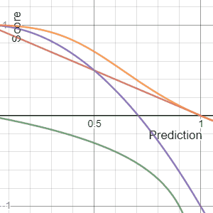
Shown below on the left is a graphical comparison of the Logarithmic, Quadratic, and Spherical scoring rules for a binary classification problem. The x-axis indicates the reported probability for the event that actually occurred.

It is important to note that each of the scores have different magnitudes and locations. The magnitude differences are not relevant however as scores remain proper under affine transformation. Therefore, to compare different scores it is necessary to move them to a common scale. A reasonable choice of normalization is shown in the picture where all scores intersect the points (0.5,0) and (1,1). This ensures that they yield 0 for a uniform distribution (two probabilities of 0.5 each), reflecting no cost or reward for reporting what is often the baseline distribution. All normalized scores below also yield 1 when the true class is assigned a probability of 1.

The scoring rules listed below aim to evaluate probabilistic predictions when the predicted distributions are univariate continuous probability distribution's, i.e. the predicted distributions are defined over a univariate target variable ${\displaystyle X\in \mathbb {R} }$ and have a probability density function ${\displaystyle f:\mathbb {R} \to \mathbb {R} _{+}}$.

The logarithmic score is a local strictly proper scoring rule. It is defined as

${\displaystyle L(D,y)=-\ln(f_{D}(y))}$

where ${\displaystyle f_{D}}$ denotes the probability density function of the predicted distribution ${\displaystyle D}$. It is a local, strictly proper scoring rule. The logarithmic score for continuous variables has strong ties to Maximum likelihood estimation. However, in many applications, the continuous ranked probability score is often preferred over the logarithmic score, as the logarithmic score can be heavily influenced by slight deviations in the tail densities of forecasted distributions.^[7]

The continuous ranked probability score (CRPS)^[8] is a strictly proper scoring rule much used in meteorology. It is defined as

${\displaystyle CRPS(D,y)=\int _{\mathbb {R} }(F_{D}(x)-H(x-y))^{2}dx}$

where ${\displaystyle F_{D}}$ is the cumulative distribution function of the forecasted distribution ${\displaystyle D}$, ${\displaystyle H}$ is the Heaviside step function and ${\displaystyle y\in \mathbb {R} }$ is the observation. For distributions with finite first moment, the continuous ranked probability score can be written as:^[1]

${\displaystyle CRPS(D,y)=\mathbb {E} _{X\sim D}[|X-y|]-{\frac {1}{2}}\mathbb {E} _{X,X'\sim D}[|X-X'|]}$

where ${\displaystyle X}$ and ${\displaystyle X'}$ are independent random variables, sampled from the distribution ${\displaystyle D}$. This is the energy form of CRPS and opens the door to estimating the CRPS via Monte Carlo sampling (through approximating the expectation value).

Furthermore, when the cumulative probability function ${\displaystyle F}$ is continuous, the continuous ranked probability score can also be written as^[9]

${\displaystyle CRPS(D,y)=\mathbb {E} _{X\sim D}[|X-y|]+\mathbb {E} _{X\sim D}[X]-2\mathbb {E} _{X\sim D}[X\cdot F_{D}(X)]}$

The continuous ranked probability score can be seen as both a continuous extension of the ranked probability score, as well as quantile regression. The continuous ranked probability score over the empirical distribution ${\displaystyle {\hat {D}}_{q}}$ of an ordered set points ${\displaystyle q_{1}\leq \ldots \leq q_{n}}$ (i.e. every point has ${\displaystyle 1/n}$ probability of occurring), is equal to twice the mean quantile loss applied on those points with evenly spread quantiles ${\displaystyle (\tau _{1},\ldots ,\tau _{n})=(1/(2n),\ldots ,(2n-1)/(2n))}$:^[10]

${\displaystyle CRPS\left({\hat {D}}_{q},y\right)={\frac {2}{n}}\sum _{i=1}^{n}\tau _{i}(y-q_{i})_{+}+(1-\tau _{i})(q_{i}-y)_{+}}$

For many popular families of distributions, closed-form expressions for the continuous ranked probability score have been derived. The continuous ranked probability score has been used as a loss function for artificial neural networks, in which weather forecasts are postprocessed to a Gaussian probability distribution.^[11][12]

CRPS was also adapted to survival analysis to cover censored events.^[13]

CRPS is also known as Cramer–von Mises distance and can be seen as an improvement of Wasserstein distance (often used in machine learning) and further Cramer distance performed better in ordinal regression than KL distance or the Wasserstein metric.^[14]

While CRPS is widely used for evaluating probabilistic forecasts, it has critical theoretical limitations. It has been shown that CRPS can produce systematically misleading evaluations by favoring probabilistic forecasts whose medians are close to the observed outcome, regardless of the actual probability assigned to that region, potentially resulting in higher scores for forecasts that allocate negligible (or even zero) probability mass to the true outcome. Furthermore, CRPS is not invariant under smooth transformations of the forecast variable, and its ranking of forecast systems may reverse under such transformations, raising concerns about its consistency for evaluation purposes.^[15]

The interval score measures the calibration and sharpness of an interval prediction ${\displaystyle (l,u)}$ at nominal coverage ${\displaystyle 1-\alpha }$:

${\displaystyle S_{\alpha }(l,u;y)=(u-l)+{\frac {2}{\alpha }}(l-y)\,\mathbf {1} \{y<l\}+{\frac {2}{\alpha }}(y-u)\,\mathbf {1} \{y>u\}}$

"The forecaster is rewarded for narrow prediction intervals, and he or she incurs a penalty, the size of which de- pends on α, if the observation misses the interval"^[16]

The scoring rules listed below aim to evaluate probabilistic predictions when the predicted distributions are univariate continuous probability distribution's, i.e. the predicted distributions are defined over a multivariate target variable ${\displaystyle X\in \mathbb {R} ^{n}}$ and have a probability density function ${\displaystyle f:\mathbb {R} ^{n}\to \mathbb {R} _{+}}$.

The multivariate logarithmic score is similar to the univariate logarithmic score:

${\displaystyle L(D,y)=-\ln(f_{D}(y))}$

where ${\displaystyle f_{D}}$ denotes the probability density function of the predicted multivariate distribution ${\displaystyle D}$. It is a local, strictly proper scoring rule.

The Hyvärinen scoring function (of a density p) is defined by^[17]

${\displaystyle s(p)=2\Delta _{y}\log p(y)+\|\nabla _{y}\log p(y)\|_{2}^{2}}$

Where ${\displaystyle \Delta }$ denotes the Hessian trace and ${\displaystyle \nabla }$ denotes the gradient. This scoring rule can be used to computationally simplify parameter inference and address Bayesian model comparison with arbitrarily-vague priors.^[17][18] It was also used to introduce new information-theoretic quantities beyond the existing information theory.^[19]

The energy score is a multivariate extension of the continuous ranked probability score:^[1]

${\displaystyle ES_{\beta }(D,Y)=\mathbb {E} _{X\sim D}[\lVert X-Y\rVert _{2}^{\beta }]-{\frac {1}{2}}\mathbb {E} _{X,X'\sim D}[\lVert X-X'\rVert _{2}^{\beta }]}$

Here, ${\displaystyle \beta \in (0,2)}$, ${\displaystyle \lVert \rVert _{2}}$ denotes the ${\displaystyle n}$-dimensional Euclidean distance and ${\displaystyle X,X'}$ are independently sampled random variables from the probability distribution ${\displaystyle D}$. The energy score is strictly proper for distributions ${\displaystyle D}$ for which ${\displaystyle \mathbb {E} _{X\sim D}[\lVert X\rVert _{2}]}$ is finite. It has been suggested that the energy score is somewhat ineffective when evaluating the intervariable dependency structure of the forecasted multivariate distribution.^[20] The energy score is equal to twice the energy distance between the predicted distribution and the empirical distribution of the observation.

The variogram score of order ${\displaystyle p}$ is given by:^[21]

${\displaystyle VS_{p}(D,Y)=\sum _{i,j=1}^{n}w_{ij}(|Y_{i}-Y_{j}|^{p}-\mathbb {E} _{X\sim D}[|X_{i}-X_{j}|^{p}])^{2}}$

Here, ${\displaystyle w_{ij}}$ are weights, often set to 1, and ${\displaystyle p>0}$ can be arbitrarily chosen, but ${\displaystyle p=0.5,1}$ or ${\displaystyle 2}$ are often used. ${\displaystyle X_{i}}$ is here to denote the ${\displaystyle i}$'th marginal random variable of ${\displaystyle X}$. The variogram score is proper for distributions for which the ${\displaystyle (2p)}$'th moment is finite for all components, but is never strictly proper. Compared to the energy score, the variogram score is claimed to be more discriminative with respect to the predicted correlation structure.

The conditional continuous ranked probability score (Conditional CRPS or CCRPS) is a family of (strictly) proper scoring rules. Conditional CRPS evaluates a forecasted multivariate distribution ${\displaystyle D}$ by evaluation of CRPS over a prescribed set of univariate conditional probability distributions of the predicted multivariate distribution:^[22]

${\displaystyle CCRPS_{\mathcal {T}}(D,Y)=\sum _{i=1}^{k}CRPS(P_{X\sim D}(X_{v_{i}}|X_{j}=Y_{j}{\text{ for }}j\in {\mathcal {C}}_{i}),Y_{v_{i}})}$

Here, ${\displaystyle X_{i}}$ is the ${\displaystyle i}$'th marginal variable of ${\displaystyle X\sim D}$, ${\displaystyle {\mathcal {T}}=(v_{i},{\mathcal {C}}_{i})_{i=1}^{k}}$ is a set of tuples that defines a conditional specification (with ${\displaystyle v_{i}\in \{1,\ldots ,n\}}$ and ${\displaystyle {\mathcal {C}}_{i}\subseteq \{1,\ldots ,n\}\setminus \{v_{i}\}}$), and ${\displaystyle P_{X\sim D}(X_{v_{i}}|X_{j}=Y_{j}{\text{ for }}j\in {\mathcal {C}}_{i})}$ denotes the conditional probability distribution for ${\displaystyle X_{v_{i}}}$ given that all variables ${\displaystyle X_{j}}$ for ${\displaystyle j\in {\mathcal {C}}_{i}}$ are equal to their respective observations. In the case that ${\displaystyle P_{X\sim D}(X_{v_{i}}|X_{j}=Y_{j}{\text{ for }}j\in {\mathcal {C}}_{i})}$ is ill-defined (i.e. its conditional event has zero likelihood), CRPS scores over this distribution are defined as infinite. Conditional CRPS is strictly proper for distributions with finite first moment, if the chain rule is included in the conditional specification, meaning that there exists a permutation ${\displaystyle \phi _{1},\ldots ,\phi _{n}}$ of ${\displaystyle 1,\ldots ,n}$ such that for all ${\displaystyle 1\leq i\leq n}$: ${\displaystyle (\phi _{i},\{\phi _{1},\ldots ,\phi _{i-1}\})\in {\mathcal {T}}}$.

All proper scoring rules are equal to weighted sums (integral with a non-negative weighting functional) of the losses in a set of simple two-alternative decision problems that use the probabilistic prediction, each such decision problem having a particular combination of associated cost parameters for false positive and false negative decisions. A strictly proper scoring rule corresponds to having a nonzero weighting for all possible decision thresholds. Any given proper scoring rule is equal to the expected losses with respect to a particular probability distribution over the decision thresholds; thus the choice of a scoring rule corresponds to an assumption about the probability distribution of decision problems for which the predicted probabilities will ultimately be employed, with for example the quadratic loss (or Brier) scoring rule corresponding to a uniform probability of the decision threshold being anywhere between zero and one. The classification accuracy score (percent classified correctly), a single-threshold scoring rule which is zero or one depending on whether the predicted probability is on the appropriate side of 0.5, is a proper scoring rule but not a strictly proper scoring rule because it is optimized (in expectation) not only by predicting the true probability but by predicting any probability on the same side of 0.5 as the true probability.^{[23][24][25][26][27][28]}

A strictly proper scoring rule, whether binary or multiclass, after an affine transformation remains a strictly proper scoring rule.^[3] That is, if ${\displaystyle S(\mathbf {r} ,i)}$ is a strictly proper scoring rule then ${\displaystyle a+bS(\mathbf {r} ,i)}$ with ${\displaystyle b\neq 0}$ is also a strictly proper scoring rule, though if ${\displaystyle b<0}$ then the optimization sense of the scoring rule switches between maximization and minimization.

A proper scoring rule is said to be local if its estimate for the probability of a specific event depends only on the probability of that event. This statement is vague in most descriptions but we can, in most cases, think of this as the optimal solution of the scoring problem "at a specific event" is invariant to all changes in the observation distribution that leave the probability of that event unchanged. All binary scores are local because the probability assigned to the event that did not occur is determined so there is no degree of flexibility to vary over.

Affine functions of the logarithmic scoring rule are the only strictly proper local scoring rules on a finite set that is not binary.

The expectation value of a proper scoring rule ${\displaystyle S}$ can be decomposed into the sum of three components, called uncertainty, reliability, and resolution,^[29][30] which characterize different attributes of probabilistic forecasts:

${\displaystyle E(S)=\mathrm {UNC} +\mathrm {REL} -\mathrm {RES} .}$

If a score is proper and negatively oriented (such as the Brier Score), all three terms are positive definite. The uncertainty component is equal to the expected score of the forecast which constantly predicts the average event frequency. The reliability component penalizes poorly calibrated forecasts, in which the predicted probabilities do not coincide with the event frequencies.

The equations for the individual components depend on the particular scoring rule. For the Brier Score, they are given by

${\displaystyle \mathrm {UNC} ={\bar {x}}(1-{\bar {x}})}$

${\displaystyle \mathrm {REL} =E(p-\pi (p))^{2}}$

${\displaystyle \mathrm {RES} =E(\pi (p)-{\bar {x}})^{2}}$

where ${\displaystyle {\bar {x}}}$ is the average probability of occurrence of the binary event ${\displaystyle x}$, and ${\displaystyle \pi (p)}$ is the conditional event probability, given ${\displaystyle p}$, i.e. ${\displaystyle \pi (p)=P(x=1\mid p)}$

• Coherence
• Decision rule

• Strictly Proper Scoring Rules, Prediction, and Estimation. Tilmann Gneiting &Adrian E Raftery Pages 359-378, https://doi.org/10.1198/016214506000001437, pdf

References

[edit]- ^ a b c d Gneiting, Tilmann; Raftery, Adrian E. (2007). "Strictly Proper Scoring Rules, Prediction, and Estimation" (PDF). Journal of the American Statistical Association. 102 (447): 359–378. doi:10.1198/016214506000001437. S2CID 1878582.
- ^ Gneiting, Tilmann (2011). "Making and Evaluating Point Forecasts". Journal of the American Statistical Association. 106 (494): 746–762. arXiv:0912.0902. doi:10.1198/jasa.2011.r10138. S2CID 88518170.
- ^ a b Bickel, E.J. (2007). "Some Comparisons among Quadratic, Spherical, and Logarithmic Scoring Rules" (PDF). Decision Analysis. 4 (2): 49–65. doi:10.1287/deca.1070.0089.
- ^ Journal of the American Statistical Association March 2007, Vol. 102, No. 477, Review Article DOI:10.1198/016214506000 Strictly Proper Scoring Rules, Prediction, and Estimation, Tilmann Gneiting and Adrian E. Raftery
- ^ Brier, G.W. (1950). "Verification of forecasts expressed in terms of probability" (PDF). Monthly Weather Review. 78 (1): 1–3. Bibcode:1950MWRv...78....1B. doi:10.1175/1520-0493(1950)078<0001:VOFEIT>2.0.CO;2.
- ^ Epstein, Edward S. (1969-12-01). "A Scoring System for Probability Forecasts of Ranked Categories". Journal of Applied Meteorology and Climatology. 8 (6). American Meteorological Society: 985–987. doi:10.1175/1520-0450(1969)008<0985:ASSFPF>2.0.CO;2. Retrieved 2024-05-02.
- ^ Bjerregård, Mathias Blicher; Møller, Jan Kloppenborg; Madsen, Henrik (2021). "An introduction to multivariate probabilistic forecast evaluation". Energy and AI. 4 100058. Elsevier BV. doi:10.1016/j.egyai.2021.100058. ISSN 2666-5468.
- ^ Zamo, Michaël; Naveau, Philippe (2018-02-01). "Estimation of the Continuous Ranked Probability Score with Limited Information and Applications to Ensemble Weather Forecasts". Mathematical Geosciences. 50 (2): 209–234. doi:10.1007/s11004-017-9709-7. ISSN 1874-8953. S2CID 125989069.
- ^ Bröcker, Jochen (2012). "Evaluating raw ensembles with the continuous ranked probability score". Quarterly Journal of the Royal Meteorological Society. 138 (667): 1611–1617. doi:10.1002/qj.1891. ISSN 0035-9009.
- ^ Rasp, Stephan; Lerch, Sebastian (2018-10-31). "Neural Networks for Postprocessing Ensemble Weather Forecasts". Monthly Weather Review. 146 (11). American Meteorological Society: 3885–3900. arXiv:1805.09091. doi:10.1175/mwr-d-18-0187.1. ISSN 0027-0644.
- ^ Grönquist, Peter; Yao, Chengyuan; Ben-Nun, Tal; Dryden, Nikoli; Dueben, Peter; Li, Shigang; Hoefler, Torsten (2021-04-05). "Deep learning for post-processing ensemble weather forecasts". Philosophical Transactions of the Royal Society A: Mathematical, Physical and Engineering Sciences. 379 (2194) 20200092. arXiv:2005.08748. doi:10.1098/rsta.2020.0092. ISSN 1364-503X. PMID 33583263.
- ^ Countdown Regression: Sharp and Calibrated Survival Predictions, https://arxiv.org/abs/1806.08324
- ^ The Cramer Distance as a Solution to Biased Wasserstein Gradients https://arxiv.org/abs/1705.10743
- ^ Beyond Strictly Proper Scoring Rules: The Importance of Being Local https://doi.org/10.1175/WAF-D-19-0205.1
- ^ Journal of the American Statistical Association March 2007, Vol. 102, No. 477, Review Article DOI 10.1198/016214506000 Strictly Proper Scoring Rules, Prediction, and Estimation, Tilmann Gneiting and Adrian E. Raftery
- ^ a b Hyvärinen, Aapo (2005). "Estimation of Non-Normalized Statistical Models by Score Matching". Journal of Machine Learning Research. 6 (24): 695–709. ISSN 1533-7928.
- ^ Shao, Stephane; Jacob, Pierre E.; Ding, Jie; Tarokh, Vahid (2019-10-02). "Bayesian Model Comparison with the Hyvärinen Score: Computation and Consistency". Journal of the American Statistical Association. 114 (528): 1826–1837. arXiv:1711.00136. doi:10.1080/01621459.2018.1518237. ISSN 0162-1459. S2CID 52264864.
- ^ Ding, Jie; Calderbank, Robert; Tarokh, Vahid (2019). "Gradient Information for Representation and Modeling". Advances in Neural Information Processing Systems. 32: 2396–2405.
- ^ Pinson, Pierre; Tastu, Julija (2013). "Discrimination ability of the Energy score". Technical University of Denmark. Retrieved 2024-05-11.
- ^ Scheuerer, Michael; Hamill, Thomas M. (2015-03-31). "Variogram-Based Proper Scoring Rules for Probabilistic Forecasts of Multivariate Quantities*". Monthly Weather Review. 143 (4). American Meteorological Society: 1321–1334. doi:10.1175/mwr-d-14-00269.1. ISSN 0027-0644.
- ^ Roordink, Daan; Hess, Sibylle (2023). "Scoring Rule Nets: Beyond Mean Target Prediction in Multivariate Regression". Machine Learning and Knowledge Discovery in Databases: Research Track. Vol. 14170. Cham: Springer Nature Switzerland. p. 190–205. doi:10.1007/978-3-031-43415-0_12. ISBN 978-3-031-43414-3.
- ^ Leonard J. Savage. Elicitation of personal probabilities and expectations. J. of the American Stat. Assoc., 66(336):783–801, 1971.
- ^ Schervish, Mark J. (1989). "A General Method for Comparing Probability Assessors", Annals of Statistics 17(4) 1856–1879, https://projecteuclid.org/euclid.aos/1176347398
- ^ Rosen, David B. (1996). "How good were those probability predictions? The expected recommendation loss (ERL) scoring rule". In Heidbreder, G. (ed.). Maximum Entropy and Bayesian Methods (Proceedings of the Thirteenth International Workshop, August 1993). Kluwer, Dordrecht, The Netherlands. CiteSeerX 10.1.1.52.1557.
- ^ Roulston, M. S., & Smith, L. A. (2002). Evaluating probabilistic forecasts using information theory. Monthly Weather Review, 130, 1653–1660. See APPENDIX "Skill Scores and Cost–Loss". [1]
- ^ "Loss Functions for Binary Class Probability Estimation and Classification: Structure and Applications", Andreas Buja, Werner Stuetzle, Yi Shen (2005) http://citeseerx.ist.psu.edu/viewdoc/summary?doi=10.1.1.184.5203
- ^ Hernandez-Orallo, Jose; Flach, Peter; and Ferri, Cesar (2012). "A Unified View of Performance Metrics: Translating Threshold Choice into Expected Classification Loss." Journal of Machine Learning Research 13 2813–2869. http://www.jmlr.org/papers/volume13/hernandez-orallo12a/hernandez-orallo12a.pdf
- ^ Murphy, A.H. (1973). "A new vector partition of the probability score". Journal of Applied Meteorology. 12 (4): 595–600. Bibcode:1973JApMe..12..595M. doi:10.1175/1520-0450(1973)012<0595:ANVPOT>2.0.CO;2.
- ^ Bröcker, J. (2009). "Reliability, sufficiency, and the decomposition of proper scores" (PDF). Quarterly Journal of the Royal Meteorological Society. 135 (643): 1512–1519. arXiv:0806.0813. Bibcode:2009QJRMS.135.1512B. doi:10.1002/qj.456. S2CID 15880012.
External links
[edit]- Video comparing spherical, quadratic and logarithmic scoring rules
- Local Proper Scoring Rules
- Scoring Rules and Decision Analysis Education
- Strictly Proper Scoring Rules
- Scoring Rules and uncertainty
- Damage Caused by Classification Accuracy and Other Discontinuous Improper Accuracy Scoring Rules
- Closed-form expressions of the continuous ranked probability score
Scoring rule
View on GrokipediaDefinitions and Fundamentals
Probabilistic Forecast
A probabilistic forecast provides a predictive probability distribution over possible future outcomes or events, rather than a single predicted value. This distribution quantifies the forecaster's uncertainty by assigning probabilities to each potential result, enabling a more complete representation of what is known or believed about the future. In contrast to point forecasts, which deliver a single deterministic value such as an expected mean, probabilistic forecasts emphasize the full spectrum of possibilities to better capture inherent uncertainties in complex systems.[5] This approach is particularly valuable in fields where decisions depend on assessing risks and ranges of outcomes, allowing users to weigh alternatives based on likelihoods. The origins of probabilistic forecasting trace back to early applications in meteorology during the early 20th century, with initial explicit treatments appearing in works like W. E. Cooke's 1906 analysis of weather predictions.[6][7] These ideas were further developed in decision theory and statistics around the mid-20th century, notably through von Neumann and Morgenstern's 1944 formulation of expected utility theory, which formalized decision-making under probabilistic uncertainty. Early meteorological uses, such as Anders Ångström's 1920s explorations of forecast value, including his 1927 and 1933 papers on probability forecasting, highlighted practical needs for probability-based predictions in weather services.[6][8] For discrete outcomes, a probabilistic forecast takes the form of a probability mass function, where probabilities sum to one across all possibilities. In continuous cases, it is represented by a probability density function. A classic example is a weather forecaster stating a 70% chance of rain tomorrow, implying a distribution over rainy and non-rainy scenarios that informs decisions like event planning. Scoring rules serve to evaluate the accuracy and calibration of such forecasts against observed outcomes.Scoring Rule
A scoring rule is a function that evaluates the quality of a probabilistic forecast given an observed outcome , assigning a numerical score where higher values indicate greater accuracy in the forecast.[1] These rules are applied in contexts such as weather forecasting, economics, and machine learning to quantify how well predicted probability distributions align with realized events.[3] In mathematical terms, a scoring rule generally takes the form , where depends only on the forecast and incorporates both the outcome and the forecast, allowing for a structured assessment of deviation from truth.[1] This structure facilitates comparisons across different forecasting methods by normalizing the evaluation process. Scoring rules serve a critical purpose in elicitation settings, where they incentivize forecasters to report their true probabilistic beliefs rather than biased estimates, thereby promoting reliable information gathering in decision-making processes.[1] The development of scoring rules traces back to the 1950s, pioneered by Glenn W. Brier in his work on verifying probability forecasts for weather events, building on foundations in statistical decision theory from earlier contributions like those of Bruno de Finetti.[3][9]Point Forecast
A point forecast provides a single predicted value for a future outcome, representing a deterministic estimate without any associated probabilities. For instance, in weather forecasting, a point forecast might predict a temperature of exactly 25°C for a given location and time, serving as a concise summary of the expected observation.[1] Such forecasts are often derived from models that optimize for a specific functional, like the mean or median, to minimize error under a chosen loss function.[10] In the framework of scoring rules, a point forecast is equivalent to a degenerate probabilistic forecast, where the predictive distribution places 100% probability mass on the single predicted value, akin to a Dirac delta distribution concentrated at that point.[1] This equivalence allows proper scoring rules designed for probabilistic forecasts—such as the continuous ranked probability score (CRPS)—to be applied directly, reducing to simpler error measures like the mean absolute error for point predictions.[1] Despite their simplicity, point forecasts have notable limitations, as they do not quantify uncertainty, potentially leading to overconfident predictions and poorer calibration in scenarios with high variability or incomplete information.[11] This omission can mislead decision-makers by implying false precision, particularly in complex domains like climate or financial modeling where outcomes are inherently stochastic.[11] Point forecasts remain prevalent in deterministic modeling approaches, such as early numerical weather prediction systems or basic regression models, where computational efficiency prioritizes a single output over distributional details.[10] Scoring rules adapt to these use cases by treating the point estimate as an implicit degenerate distribution, enabling consistent evaluation alongside more expressive probabilistic forecasts.[1]Scoring Function
A scoring function constitutes the foundational mathematical construct for assessing the quality of probabilistic forecasts by comparing a predicted distribution to a realized outcome. Denoted typically as , where is the observed outcome and is the forecasted probability distribution, it maps these inputs to a real number that quantifies their correspondence. This structure underpins the evaluation process in probabilistic forecasting, serving as the atomic unit from which broader assessment mechanisms are built.[1] For discrete outcomes over a finite sample space, the scoring function takes the basic form , where represents the realized outcome and is the vector of forecasted probabilities assigned to each possible event. In the continuous setting, involving probability densities , the function evaluates the forecast at the outcome , with the integral form capturing its expectation under the forecasted density; this integral provides the theoretical basis for averaging scores across potential realizations. These algebraic expressions ensure the function's applicability across diverse probabilistic domains without presupposing specific distributional assumptions.[12] Scoring functions possess general properties that enhance their utility in forecast evaluation, including monotonicity with respect to forecast accuracy—scores improve (non-decreasing in positive orientation or non-increasing in negative) as the forecasted distribution aligns more closely with the true underlying probabilities. They are not inherently required to satisfy stricter conditions like propriety, allowing flexibility in design while prioritizing sensitivity to discrepancies between forecast and outcome. Orientation influences whether higher numerical values indicate better performance (positive) or worse (negative), a choice that standardizes interpretation in applications.[1] In contrast to fully specified scoring rules, which involve the operational deployment of these functions—such as aggregation over samples or integration into decision frameworks—scoring functions remain the elemental components focused solely on pairwise evaluation of outcome and forecast. This distinction underscores their role as versatile building blocks rather than complete verification protocols.[13]Orientation of Scoring Rules
Scoring rules are classified by their orientation, which determines whether higher or lower numerical values indicate superior forecast performance. Positively oriented scoring rules reward accurate probabilistic forecasts with higher scores, such as the logarithmic scoring rule, where the score is the logarithm of the predicted probability assigned to the observed outcome, and forecasters aim to maximize the expected value. In contrast, negatively oriented scoring rules function as penalties, assigning lower values (often closer to zero or more negative) to better forecasts; the Brier score, defined as the mean squared difference between predicted probabilities and binary outcomes, exemplifies this by penalizing deviations and is minimized for optimal performance. The orientation of a scoring rule can be inverted without altering its relative evaluation of forecasts: multiplying the rule by −1 flips it from positive to negative (or vice versa), preserving the ordering of forecast quality since the transformation is monotonic. This equivalence ensures that core properties like propriety remain intact under sign reversal. The choice of orientation carries practical implications for applications. Positively oriented rules align with elicitation contexts, where forecasters maximize expected scores to reveal true beliefs, a framework rooted in decision theory. Negatively oriented rules predominate in machine learning optimization, treating scores as loss functions to minimize during model training, facilitating integration with gradient-based algorithms. This convention of distinguishing orientations emerged as standard in the probabilistic forecasting literature since the 1970s, though usage varies by discipline—positive in statistics and meteorology, negative in computational fields.Expected Score
The expected score serves as the theoretical performance metric for a scoring rule, quantifying the long-run average score a forecaster would receive if repeatedly issuing the same probabilistic forecast under a true underlying distribution. For a forecast distribution and true distribution over a discrete sample space, the expected score is defined as where is the score assigned to the forecast upon observing outcome . This expectation represents the mean score over outcomes drawn from .[1] In the continuous case, the expected score takes the integral form where the integration is over the sample space, and denotes the forecasted density or cumulative distribution function evaluated at . This formulation extends the discrete case to handle outcomes from continuous distributions, maintaining the focus on average performance relative to the true distribution .[1] The expected score plays a central role in evaluating forecast quality, as it measures the anticipated long-run performance of a scoring rule. For proper scoring rules, the expected score is maximized when the forecast equals the true distribution , incentivizing forecasters to report their true beliefs to achieve the highest possible average score. Strict propriety further strengthens this by ensuring that the maximum is unique, attained only when , which promotes unambiguous truthful reporting in probabilistic forecasting.[1]Sample Average Score
The sample average score, also referred to as the empirical score, quantifies the performance of probabilistic forecasts by averaging the values of a scoring rule over a finite set of forecast-observation pairs. For pairs , where denotes the observed outcome and the forecast distribution at occasion , it is defined as with representing the scoring rule. This measure was introduced in early forecast verification studies within meteorology, notably in Brier's 1950 analysis of probabilistic weather predictions, where it served as a mean squared error metric to assess forecast accuracy across multiple events.[3] Assuming the pairs are independent and identically distributed, the sample average score is an unbiased estimator of the expected score, meaning its expectation equals the true population value. Furthermore, under standard regularity conditions such as finite variance, it converges almost surely to the expected score as the sample size approaches infinity, by the law of large numbers; this consistency property ensures that long-term empirical performance reliably reflects theoretical quality. In practice, the sample average score facilitates forecaster evaluation and model selection using finite datasets, where competing methods are ranked by their aggregated scores—typically favoring those with minimal values for negatively oriented rules—to identify superior predictive systems without awaiting infinite data. This data-driven approach bridges theoretical expected scores to operational decision-making, though finite-sample variability necessitates careful sample size considerations for robust comparisons.Properties and Theoretical Foundations
Proper Scoring Rules
A proper scoring rule is a mechanism for evaluating probabilistic forecasts such that the expected score is maximized when the forecaster reports their true belief distribution. Formally, for a scoring rule that assigns a score based on reported probabilities and observed outcome , and true probability distribution , the rule is proper if the expected score satisfies for all probability distributions . This property ensures that, under the true distribution, no other report yields a higher expected score than truthful reporting. Strict propriety strengthens this condition by guaranteeing a unique maximum at the true distribution, meaning the inequality is strict unless . This unique incentive aligns the forecaster's optimal strategy precisely with honesty, eliminating any ambiguity in the reporting equilibrium. The theoretical foundations of proper scoring rules trace back to decision theory in the mid-20th century, with Leonard Savage's 1971 work providing a seminal characterization linking them to expected utility maximization and subjective probability elicitation.[14] Savage demonstrated that proper scoring rules correspond to convex functions on probability simplices, enabling their use as devices to infer personal probabilities without strategic distortion, building on earlier ideas from de Finetti's coherence axioms. In practice, proper scoring rules facilitate truthful elicitation of beliefs in uncertain environments, preventing strategic misrepresentation by making dishonesty suboptimal in expectation. This has profound implications for applications like forecast verification and incentive-compatible mechanisms in economics and statistics.Strictly Proper Scoring Rules
A strictly proper scoring rule is a refinement of a proper scoring rule, where the expected score under the true distribution is uniquely maximized by reporting itself. Formally, for a scoring rule , it is strictly proper if for all probability distributions .[1] This strict inequality ensures that any deviation from the true forecast results in a strictly lower expected score, incentivizing precise calibration and sharpness in probabilistic forecasts.[1] In contrast to merely proper scoring rules, which allow multiple forecasts to achieve the maximum expected score, strictly proper rules eliminate such ambiguity, making them particularly valuable for eliciting truthful and unique probabilistic predictions.[1] Examples of proper but not strictly proper scoring rules include the zero-one score, which assigns a score of 1 if the forecast's mode matches the outcome and 0 otherwise; this is proper because the expected score is maximized by any forecast assigning positive probability only to the true outcome, but it is not strictly proper due to non-uniqueness among such forecasts.[1] Similarly, the energy score with parameter is proper for distributions with finite second moments but not strictly proper, as multiple forecasts can yield the same expected score.[1] Such non-strict rules are rare in practice, as they often fail to distinguish between equally calibrated but differently sharp forecasts.[1] The strict propriety of a scoring rule follows from the strict convexity of the negative expected score function with respect to the forecast distribution. Specifically, the negative expected score is a strictly convex function of , implying a unique minimum at .[1] This convexity links strictly proper scoring rules to Bregman divergences, where the divergence generated by a strictly convex function defines the negative expected score as , ensuring the strict inequality for .[1] A brief proof sketch involves Jensen's inequality applied to the strictly convex : for , the convexity yields , leading directly to the strict maximization of the expected score at .[1] Most commonly used scoring rules in forecasting and statistics are strictly proper, including the logarithmic score and the Brier (quadratic) score.[1] For instance, the logarithmic score, defined as , is strictly proper for both discrete and continuous distributions, uniquely rewarding the true probabilities.[1] Likewise, the Brier score for categorical outcomes, , is strictly proper, providing a quadratic penalty that penalizes deviations from the true distribution.[1] These properties make strictly proper rules the standard for applications requiring robust evaluation of probabilistic forecasts.[1]Consistent Scoring Functions
In statistics, a consistent scoring function provides a framework for evaluating point forecasts of specific distributional functionals, ensuring that the scoring rule incentivizes accurate estimation of those functionals. Formally, consider a space of possible outcomes, a space of forecasts, and the set of probability distributions over . A functional maps distributions to point estimates, such as the mean or a quantile. A scoring function is consistent for if, for any distribution and random outcome , with the infimum achieved uniquely at for strict consistency. This property implies that the expected score is minimized precisely when the forecast equals the true functional value, promoting truthful reporting.[15] In practice, with an observed sample , the sample average score serves as an estimator. Under suitable regularity conditions, such as convexity of and continuity of , the minimizer converges almost surely to as , making consistent scoring functions a basis for asymptotically valid point estimation. This convergence underpins their utility in empirical forecast verification, where the sample average approximates the population minimization.[15] Proper scoring rules, which evaluate full probabilistic forecasts, represent a special case of consistent scoring functions where the functional is the identity mapping, i.e., , directly eliciting the true distribution.[15] Classic examples illustrate this framework. The squared error score is strictly consistent for the mean functional , as its expected value (with ) is uniquely minimized at . Similarly, the mean absolute error is strictly consistent for the median functional , since the expected absolute deviation is minimized at the median for any distribution. These examples extend to other functionals like quantiles and expectiles, where consistent scores can be constructed via integral representations.[15] The general theory of consistent scoring functions was formalized in the statistics literature during the 2010s, building on earlier work in decision theory to address challenges in verifying point forecasts for complex functionals in fields like meteorology and econometrics. Seminal contributions, including characterizations via Choquet integrals and forecast rankings, have established their role in ensuring robust evaluation beyond simple location parameters.[15]Applications in Practice
Weather and Climate Forecasting
Scoring rules have played a pivotal role in the verification of probabilistic forecasts in meteorology since the mid-20th century, particularly for assessing the accuracy of predictions in weather and climate contexts. The Brier score, originally proposed in 1950, was developed specifically for evaluating probabilistic forecasts of binary events, such as the occurrence or non-occurrence of precipitation, providing a quadratic measure of forecast accuracy that penalizes deviations from observed outcomes.[3] For continuous predictands like temperature or wind speed, the Continuous Ranked Probability Score (CRPS) emerged in the 1970s as a key metric, generalizing the mean absolute error to probabilistic distributions and enabling fair comparisons between deterministic and ensemble forecasts.[16] In operational settings, such as those at the European Centre for Medium-Range Weather Forecasts (ECMWF), scoring rules are routinely applied to evaluate ensemble prediction systems for variables including surface temperature and precipitation. The Discrete Ranked Probability Score (RPS) is used for categorical forecasts, measuring the cumulative differences between predicted and observed cumulative probabilities across ordered categories,[17] while the CRPS assesses continuous forecasts by integrating the squared differences between predictive and empirical cumulative distribution functions derived from ensembles. These metrics are computed over verification periods using reanalysis datasets like ERA5, allowing forecasters to quantify performance across lead times from short-range to medium-range predictions.[18] The primary benefits of these scoring rules in weather forecasting lie in their ability to simultaneously evaluate calibration—the statistical reliability of predicted probabilities—and sharpness—the concentration of predictive distributions around expected outcomes—thus incentivizing forecasts that are both accurate and informative.[19] By rewarding proper probabilistic reporting, they facilitate the construction of skill scores, such as the Ranked Probability Skill Score (RPSS), which normalize raw scores against climatological benchmarks to highlight relative improvements in forecast quality. By the 2020s, scoring rules had become embedded in the verification processes for large-scale climate model intercomparisons, including Phase 6 of the Coupled Model Intercomparison Project (CMIP6), where the Brier Skill Score is applied to assess the performance of global climate models in simulating seasonal precipitation patterns against observational data.[20] This integration supports model selection and bias correction in projections of future climate variability, enhancing the reliability of assessments for decision-making in sectors like agriculture and water resource management.Economic and Decision Theory
In economic and decision theory, proper scoring rules play a crucial role in eliciting truthful subjective probabilities from individuals in settings such as markets and surveys, ensuring that reported beliefs maximize the expected reward under risk neutrality. These rules incentivize honest reporting by assigning scores that peak when the forecaster's probability distribution matches their true beliefs, thereby facilitating the aggregation of dispersed information for collective decision-making.[1] Applications of scoring rules in economics include prediction markets, where mechanisms like the logarithmic market scoring rule (LMSR) enable continuous trading and probability updates without requiring matched counterparties, promoting efficient information revelation. For instance, the Iowa Electronic Markets, a long-running real-money platform for forecasting elections and economic events, leverages market-based incentives akin to scoring rules to aggregate participant beliefs into accurate consensus probabilities. In cost-benefit analysis, scoring rules aid in quantifying uncertainty by eliciting probabilistic assessments of outcomes, allowing decision-makers to compute expected net benefits under alternative scenarios.[21][22] A key theoretical link exists between scoring rules and utility maximization: for a risk-neutral agent, the expected score from a proper rule aligns precisely with the expected utility derived from acting on the true probability distribution, making truthful reporting the optimal strategy in Bayesian decision frameworks. This connection underpins their use in behavioral economics for modeling subjective expectations.[1] The prominence of scoring rules in economic applications grew in the 1990s and 2000s within behavioral economics, particularly through Charles Manski's work on measuring subjective probabilities via incentivized elicitation methods that address biases in survey responses. Manski emphasized their potential to reveal full probability distributions rather than point estimates, enhancing econometric analysis of decision-making under uncertainty.[23]Machine Learning and Calibration
In machine learning, proper scoring rules serve as loss functions for training probabilistic classifiers and regressors, incentivizing models to output calibrated probability distributions. The logarithmic scoring rule, equivalent to the cross-entropy loss, is widely used in neural networks for multi-class classification, where it minimizes the negative log-likelihood of the true class under the predicted probability distribution.[24] This loss function encourages the model to assign high probabilities to correct classes and low probabilities to incorrect ones, facilitating gradient-based optimization in deep learning frameworks. Similarly, the Brier score, or quadratic scoring rule, functions as a mean squared error loss for multi-class settings by penalizing deviations between predicted probabilities and one-hot encoded true labels across all classes.[24] Both rules are strictly proper, ensuring that the model's expected loss is minimized only when its predictions match the true conditional distribution, which supports reliable probabilistic outputs in supervised learning tasks.[1] Scoring rules are instrumental in evaluating and improving model calibration, a critical aspect of trustworthy artificial intelligence where predicted probabilities should reflect true empirical frequencies. The expected calibration error (ECE) quantifies miscalibration by binning predictions based on confidence and measuring the difference between average predicted probabilities and observed accuracies within each bin, often using sample averages of proper scoring rules like the Brier or logarithmic score to estimate reliability.[25] Poor calibration, detectable through high ECE values, can lead to overconfident or underconfident predictions, undermining applications in high-stakes domains such as medical diagnosis or autonomous systems; thus, post-hoc recalibration techniques, informed by these scores, adjust model outputs to align confidence with accuracy.[25] In trustworthy AI, proper scoring rules provide a unified framework for assessing not just accuracy but also the sharpness and resolution of probabilistic forecasts, ensuring models are both precise and reliable.[24] Recent developments in the 2020s have extended scoring rules to uncertainty quantification in large language models (LLMs), where they evaluate the decomposition of total uncertainty into aleatoric (data-inherent) and epistemic (model-induced) components. For instance, frameworks using proper scores like the Brier and logarithmic rules have improved calibration in LLMs for tasks such as clinical text classification, reducing Brier scores by up to 74% and enhancing expected calibration error through Bayesian-inspired approximations of posterior distributions.[26] Methods leveraging proper scoring rules also guide selective prediction and out-of-distribution detection by tailoring uncertainty estimates to task-specific losses for better performance in real-world deployment.[27] A key theoretical link exists between proper scoring rules and Bayesian methods, where the expected logarithmic score under the true distribution equals the negative Shannon entropy minus the Kullback-Leibler (KL) divergence to the predicted distribution, implying that proper rules minimize KL divergence when predictions align with the true posterior.[1] This connection underpins their use in variational inference and Bayesian neural networks, promoting forecasts that are information-theoretically optimal.Examples of Proper Scoring Rules
Logarithmic Score for Categorical and Continuous Variables
The logarithmic scoring rule, also known as the log score or ignorance score, evaluates probabilistic forecasts by assigning a score based on the logarithm of the predicted probability assigned to the observed outcome. For categorical variables with a finite set of outcomes, the score is defined as where is the realized outcome and is the forecaster's assigned probability to that outcome, assuming a positive orientation where higher scores indicate better performance. This formulation originates from early work on admissible probability measurement procedures, where it was identified as the unique local strictly proper scoring rule. For continuous variables, the logarithmic score extends naturally to probability densities, given by where denotes the predicted probability density function and is the observed value. In both discrete and continuous cases, the score is undefined if the predicted probability or density at the outcome is zero, which underscores its strict requirement for positive support across possible outcomes.[28] The logarithmic score is strictly proper, meaning that the expected score is uniquely maximized when the forecaster reports their true subjective probabilities, incentivizing honesty without strategic misrepresentation. It elicits the geometric mean in aggregation contexts, such as pooling multiple forecasts, where the optimal combined probability corresponds to the weighted geometric mean of individual predictions under this rule.[29] Additionally, the score is particularly sensitive to low-probability assignments; assigning a very small probability to the realized outcome results in a large negative score, heavily penalizing underestimation of rare events.[2] The derivation of the logarithmic score's propriety follows from information theory, where the expected score under true probabilities for a forecast is in the discrete case (or the integral analog for continuous), which simplifies to the negative Shannon entropy minus the Kullback-Leibler divergence: . This expression is maximized uniquely when , as the KL divergence is zero only for matching distributions, thereby linking the score's optimization to entropy maximization.Brier and Quadratic Scores
The Brier score is a quadratic scoring rule originally developed for evaluating probabilistic forecasts in meteorology. Introduced by Glenn W. Brier in 1950, it was proposed as a method to verify weather predictions expressed in terms of probabilities, such as the likelihood of precipitation, by measuring the mean squared difference between forecasted probabilities and observed binary outcomes. This score has since become a standard metric in forecast verification across various fields, rewarding forecasts that align closely with observed events while penalizing deviations.[1] For a categorical prediction with possible outcomes, let denote the forecasted probability vector, where and , and let be the realized outcome. The indicator vector has , which equals 1 if outcome occurs and 0 otherwise. The Brier score is then given by where is the squared Euclidean norm. This negative orientation treats the score as a reward, with higher (less negative) values indicating superior forecast accuracy; equivalently, the positive version functions as a loss, minimized for accurate predictions.[1] For a sequence of independent forecasts, the overall score is the average . The Brier score possesses key theoretical properties that underpin its utility. It is a strictly proper scoring rule: for any true probability distribution , the expected score is uniquely maximized when , incentivizing forecasters to report their true beliefs rather than hedging or biasing probabilities.[1] Additionally, it is decomposable, permitting the expected score to be partitioned into terms capturing calibration (the reliability of predicted probabilities relative to observed frequencies) and refinement (the sharpness or variability of the forecasts, reflecting their informativeness). Specifically, the expected Brier score can be expressed as , where is the uncertainty inherent in the observations (a fixed climatological term), is the resolution or refinement (higher for sharper forecasts), and is the calibration error (lower for well-calibrated forecasts); this decomposition, originally due to Murphy, highlights trade-offs in forecast quality.[30] As a quadratic form, the Brier score generalizes naturally to point forecasts. When the probability vector is degenerate—assigning probability 1 to a single predicted outcome and 0 elsewhere—the score simplifies to , the negative squared error between the point prediction and the actual outcome. This connection positions the Brier score as an extension of the classical quadratic loss function to probabilistic settings, bridging deterministic and uncertain forecasting paradigms.[1]Spherical Score
The spherical score is a strictly proper scoring rule designed for evaluating probabilistic forecasts over categorical outcomes, where the forecast is represented by a probability vector with and , and the outcome is indicated by a one-hot vector such that and for . It can be expressed in vector form as the dot product of the forecast and outcome vectors, normalized by the Euclidean norm of the forecast vector: An alternative formulation, which scales the score differently while preserving its propriety, is . This rule assigns higher scores (closer to 1) for forecasts that align well with the observed outcome, with the maximum score of 1 achieved when is a Dirac delta at . The spherical score is strictly proper, meaning that for any true probability distribution , the expected score is uniquely maximized when the forecast . It belongs to a family of power-based scoring rules derived from Bregman divergences associated with the -norm for , ensuring that deviations from the true distribution are penalized in a convex manner. Regarding transformations, the spherical score's expected value under the true distribution remains invariant under positive affine transformations of the score function, a property shared by all proper scoring rules, which preserves its incentive compatibility for eliciting honest forecasts.[31] Geometrically, the spherical score interprets the probability vector as a point in the probability simplex, projected onto the unit sphere in via normalization by . The score then measures the cosine of the angle between this projected vector and the outcome direction , rewarding forecasts that are both concentrated (higher ) and correctly aligned with the outcome.[31] This projection emphasizes directional accuracy over magnitude, making it particularly suitable for distinguishing forecasts in scenarios where probability mass is spread across many categories. Although less commonly applied than the logarithmic or Brier scores, the spherical score finds utility in high-dimensional categorical settings, such as multi-class classification or ensemble forecasting with numerous outcomes, where its normalization helps evaluate relative alignments without excessive sensitivity to the overall entropy of the forecast distribution.Ranked Probability Score
The Ranked Probability Score (RPS) is a strictly proper scoring rule specifically developed for evaluating probabilistic forecasts of ordered categorical outcomes, such as severity levels or ranked events. Introduced by Epstein in 1969, it extends the Brier score by incorporating the ordinal structure of categories, thereby addressing limitations in scores that ignore ranking. This makes the RPS particularly useful for applications where the relative positions of categories matter, like weather intensity forecasts or economic indicators on ordinal scales.[32][1] The RPS is computed based on the cumulative distribution functions of the forecast and observation. For ordered categories, let denote the forecasted cumulative probability up to category (i.e., the probability that the outcome is category or lower), and the corresponding observed cumulative indicator (0 if the outcome exceeds category , 1 otherwise). The score is given by: Lower values indicate better forecast accuracy, with the minimum value of 0 achieved when the forecast perfectly matches the observation. This formulation normalizes the score to the range [0, 1], facilitating comparisons across different numbers of categories.[32][1] As a strictly proper rule, the RPS incentivizes forecasters to report their true subjective probabilities, minimizing the expected score only when the forecast distribution matches the true one. It penalizes rank errors by quadratically weighting discrepancies in cumulative probabilities, with larger penalties for misplacements farther apart in the ordering—for instance, confusing the lowest and highest categories incurs a higher cost than adjacent ones. Compared to the Brier score, which evaluates each category independently and thus underutilizes ordinal information, the RPS provides a more nuanced assessment for ordered data, improving interpretability in contexts like multi-level risk assessments.[1][33] In practice, the RPS has found application in economics, particularly for verifying survey-based density forecasts of variables like inflation or GDP growth, where ordinal categorizations are common. Its sensitivity to cumulative misalignments helps highlight both calibration and resolution in such forecasts, though it assumes equal spacing between categories unless weights are incorporated. Seminal analyses confirm its robustness as an extension of quadratic scoring rules from the 1970s, balancing simplicity with ordinal awareness.[33][1]Continuous Ranked Probability Score
The Continuous Ranked Probability Score (CRPS) is a strictly proper scoring rule designed to evaluate univariate probabilistic forecasts expressed as cumulative distribution functions (CDFs). It measures the squared L2 distance between the forecast CDF and the Heaviside step function corresponding to the observed value , providing a comprehensive assessment of forecast sharpness and calibration.[1] The CRPS is defined as where is the indicator function. This integral form generalizes the mean absolute error to distributional forecasts, reducing to the absolute error when is a degenerate distribution at a point forecast . As a strictly proper score, the CRPS is minimized in expectation when the forecast CDF matches the true conditional distribution, incentivizing honest probabilistic predictions.[1] For computation, the CRPS lacks a universal closed-form expression but can be evaluated efficiently using numerical quadrature methods, particularly for parametric distributions like the Gaussian, where explicit formulas exist involving the cumulative distribution function and density : When forecasts are represented by samples, an algorithm based on order statistics provides an unbiased estimate. Advanced methods link the CRPS to distances in reproducing kernel Hilbert spaces via kernel mean embeddings, enabling scalable computation for complex distributions.[1] Since the early 2000s, the CRPS has become a standard metric in meteorology for verifying ensemble weather forecasts, decomposing into components of reliability, resolution, and uncertainty to diagnose forecast performance. In hydrology, it is widely applied to assess probabilistic predictions of variables like river discharge and precipitation, supporting model calibration and intercomparison.[34][35]Energy and Variogram Scores for Multivariate Cases
The energy and variogram scores provide essential tools for evaluating multivariate probabilistic forecasts of continuous joint distributions, capturing dependencies across dimensions that univariate scores cannot address. These scores are particularly valuable in fields requiring assessment of spatial or temporal correlations, such as climate modeling, where forecasts often involve vector-valued outcomes like temperatures or wind speeds at multiple locations. The energy score measures the discrepancy between a forecast distribution and an observation using Euclidean distances between random draws. It is given by where denotes the Euclidean norm and the expectations are with respect to independent draws from . This formulation ensures the score is strictly proper, as the expected score is minimized when , the true distribution. In practice, the score is estimated via Monte Carlo integration using samples from , making it suitable for ensemble-based forecasts. The energy score was introduced as a multivariate generalization of the continuous ranked probability score and has kernel representations linking it to negative definite functions. When comparing two distributions via samples and , an analogous form of the energy distance is which quantifies divergence and equals zero if and only if (under mild conditions). For a single observation (, ), this reduces to the energy score up to scaling. The score is elicitable for the multivariate mean in the sense that it penalizes deviations in location parameters. Developed in the mid-2000s, the energy score saw increased adoption in the 2010s for verifying ensemble forecasts in meteorology and climate science. The variogram score, inspired by the semivariogram in geostatistics, extends similar ideas by incorporating powers of distances to assess dependence structures. The core component is the variogram of order , defined as , where are independent draws from the distribution and typically or . The scoring rule compares the forecast's expected variogram to an empirical version from the observation, often in the form This generalizes the energy score (which corresponds to ) and is strictly proper under stationarity assumptions on the underlying process, ensuring the expected score is optimized for truthful forecasts. The variogram score is particularly sensitive to misspecifications in variances and correlations, and it elicits the mean vector by being minimized at the correct location parameters. Introduced in the 2010s specifically for multivariate probabilistic forecasts in spatial and temporal contexts, it has been applied to climate variables like wind speeds across sites, aiding diagnosis of ensemble underdispersion or correlation errors.[36] Both scores facilitate interpretation of proper scoring rules by decomposing forecast errors into components related to location, spread, and dependence, though they require careful normalization for comparability across dimensions.[36]Comparison and Interpretation of Proper Scoring Rules
Proper scoring rules, while all incentivizing honest reporting of probabilistic forecasts, differ in their sensitivity to various aspects of forecast quality, such as calibration, sharpness, and tail behavior. For instance, the logarithmic score is highly sensitive to extreme probabilities, penalizing overconfident predictions in the tails more severely than the Brier score, which emphasizes overall mean squared error and is more forgiving of calibration errors.[37][1] In contrast, the continuous ranked probability score (CRPS) is robust to outliers but less sensitive to multivariate dependency structures compared to the energy score, which better detects errors in joint distributions.[38] These differences affect interpretability, as scores like the Brier provide decomposable insights into reliability and resolution, aiding diagnostic analysis.[39] All strictly proper scoring rules are equivalent up to positive affine transformations for the purpose of elicitation, meaning they yield the same optimal forecast distribution under expectation, but they diverge in robustness and practical utility.[1] For example, while the logarithmic score's sensitivity to low-probability events makes it ideal for emphasizing sharpness, the CRPS offers greater robustness in continuous settings by integrating over the full cumulative distribution.[38] This equivalence ensures consistent incentives, yet non-equivalence in finite samples or under misspecification highlights the need for rule-specific interpretations, such as the energy score's strength in multivariate robustness despite higher computational demands.[38] The choice of a proper scoring rule depends on the forecasting domain and data characteristics. In categorical settings, the Brier or logarithmic scores are preferred for their direct handling of discrete outcomes and ease of decomposition.[1] For continuous variables, the CRPS suits univariate cases by evaluating the entire distribution, while the energy score excels in multivariate scenarios where dependencies matter.[38] Ordered data may favor scores like the ranked probability score for preserving ordinal structure, whereas unordered multivariate data benefits from kernel-based approaches like the energy score.[1]| Scoring Rule | Sensitivity Characteristics | Computability Notes | Typical Domain Suitability |